New Applications of Bradley Terry Models
A Bradley Terry model ranks opponents to give a probability that a match up will lead to a win or loss for either team. Draws are not allowed in the most basic Bradley Terry (BT) model, which makes them impractical for football results. There are extensions that allow for draws, (here), but in this post I will show how we formulated our own ‘games’ in football for which a BT model can be used.
As a side project I predict red cards in football and host my results at www.illiquidodds.com. Therefore I’m always on the look out for new ways to see how we can model a red card occurring in a match. What if we can formulate a football match as a competition between two teams where a win is counted as getting a member of the other team sent off. Each match, i.e. Tottenham vs Arsenal can be broken down into two separate matches. One where Tottenham competes to get an Arsenal player sent off and another where Arsenal competes to get a Tottenham player sent off.
Then using this new dataset we can fit a BT model to see who is better at getting someone from the other team sent off.
e0 <- read_csv("E0_1718.csv")
e0$MatchID <- seq_len(nrow(e0))
uniqTeams <- unique(c(e0$HomeTeam, e0$AwayTeam))
We classify 1 as a win. As 314 matches have been played, this means that we’ve actually 628 different red card games. Using dplyr we can easily manipulate the raw data into a training frame for our model.
e0 %>% select(Date, MatchID, HomeTeam, AwayTeam, HR, AR) %>% rename(team1=HomeTeam, team2=AwayTeam) %>% mutate(Red=as.numeric(AR > 0)) -> homeWins
e0 %>% select(Date, MatchID, HomeTeam, AwayTeam, HR, AR) %>% rename(team1=AwayTeam, team2=HomeTeam) %>% mutate(Red=as.numeric(HR > 0)) -> awayWins

bind_rows(homeWins, awayWins) %>% mutate(Date=dmy(Date), team1=factor(team1, levels = uniqTeams), team2=factor(team2, levels = uniqTeams)) -> trainData
We will be using a Bayesian Bradley-Terry model from http://opisthokonta.net/?p=1589. We will be using an uninformative prior on the ratings. There is no prior knowledge at the start of the season that we could reasonably incorporate into the model. As we are also interested in just the team rankings, it seems more appropriate that they all start with the same rank.
options(mc.cores=1)
stanModel <- stan_model("bt_redcard.stan")

stanData <- list()
stanData$N <- nrow(trainData)
stanData$P <- length(uniqTeams)
stanData$team1 <- as.numeric(trainData$team1)
stanData$team2 <- as.numeric(trainData$team2)
stanData$results <- trainData$Red
stanData$alpha <- rep_len(1, stanData$P)

smpls <- sampling(stanModel, stanData)
There are no issues in sampling with plenty of effective samples emerging. When we plot the ratings we find some interesting results.
fit <- as.matrix(smpls)
plot(smpls, pars=c("ratings")) + scale_y_continuous(labels=uniqTeams, breaks=rev(seq_along(uniqTeams))) + geom_vline(xintercept = 1/length(uniqTeams))
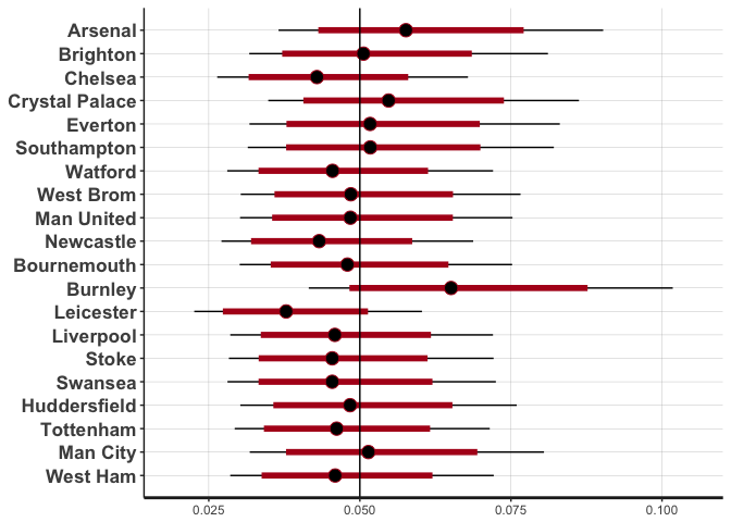
Most of the teams do not differ that much from the actual prior distribution, indicated by the black line at 0.05. This means that guessing whether a team with rating 0.05 will get someone on the other team sent off is no better than a coin flip, i.e. 50%. But there are some teams that stand out as quite different from this mean. Burnley and Arsenal have higher ratings, which means they are better than average at getting a player from the other team sent off. Burnley have been overachieving this season, could this be a potential explainer? Teams with a lower ranking, such as Leicester, have not succeed in getting the other team a red card.
Leicester’s Title Winning Season
In the 2015-1016 Leicester City defied all odds to win the Premier League for the first time in their history. Could the amount of red cards the other teams received against them had anything to do with this?
e0 <- read_csv("E0_1516.csv")

e0$MatchID <- seq_len(nrow(e0))
uniqTeams <- unique(c(e0$HomeTeam, e0$AwayTeam))

e0 %>% select(Date, MatchID, HomeTeam, AwayTeam, HR, AR) %>% rename(team1=HomeTeam, team2=AwayTeam) %>% mutate(Red=as.numeric(AR > 0)) -> homeWins
e0 %>% select(Date, MatchID, HomeTeam, AwayTeam, HR, AR) %>% rename(team1=AwayTeam, team2=HomeTeam) %>% mutate(Red=as.numeric(HR > 0)) -> awayWins

bind_rows(homeWins, awayWins) %>% mutate(Date=dmy(Date), team1=factor(team1, levels = uniqTeams), team2=factor(team2, levels = uniqTeams)) -> trainData

stanModel <- stan_model("bt_redcard.stan")

stanData <- list()

stanData$N <- nrow(trainData)
stanData$P <- length(uniqTeams)
stanData$team1 <- as.numeric(trainData$team1)
stanData$team2 <- as.numeric(trainData$team2)
stanData$results <- trainData$Red
stanData$alpha <- rep_len(1, stanData$P)

smpls <- sampling(stanModel, stanData)

fit <- as.matrix(smpls)
plot(smpls, pars=c("ratings")) + scale_y_continuous(labels=uniqTeams, breaks=rev(seq_along(uniqTeams))) + geom_vline(xintercept = 1/length(uniqTeams))
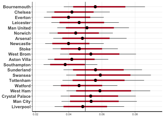
We can see that Leicester was below the average. So their title win was unlikely to be because of their ability to get someone sent off. However, Newcastle, Norwich and Aston Villa are quite far below the average also. These were the three worst teams in the Premier League and subsequently got relegated, so perhaps the sending offs didn’t go their way throughout the season, which led to missed points.
Overall, the actual usefulness of this type of model is questionable. It appears to be descriptive and allows us to compare teams on their ability to get the other team sent off, but how well this works as a predictive model is very dubious. Still, it’s a nice foray into Bradley Terry models and shows how easy they can be fitted using Stan.