Non Parametric Priors with Dirichlet Processes
One of the main benefits of my R package dirichletprocess is the
ability to drop in the objects it creates as components of models. In
this blog post I will show you how you can use a Dirichlet process as a
prior distribution of a parameter in a Bayesian model.
Enjoy these types of posts? Then sign up for my newsletter.
require(dplyr)
require(knitr)
require(ggplot2)
require(dirichletprocess)
require(rstan)
require(tidyr)
Rats!
The data we will be using consists of 71 experiments where \(N\) rats are given a drug and \(y\) are found to have developed tumours.
rats %>% sample_n(4) %>% kable
| y | N |
|---|---|
| 2 | 24 |
| 6 | 22 |
| 3 | 27 |
| 1 | 18 |
We want to model \(\theta = \frac{y}{N}\), which is the rate of tumours in each experiment.
The Basic Bayesian Model
In the most basic model, we can assume that the the rats with tumours are Binomially distributed at a rate of \(\theta\), which can be written as:
\[\begin{aligned} y_i & \sim \text{Binomial} (N_i, \theta _i), \\ \theta_i & \sim \text{Beta} (\alpha _0, \beta _0). \\ \end{aligned}\]We then assume that there is only one \(\theta\) and it applies to each experiment. As this is a conjugate model, we can easily apply Bayes theorem and arrive at a analytical posterior.
\[\begin{aligned} \theta & \mid y_i, N_i \sim \text{Beta} (\alpha , \beta), \\ \alpha & = \alpha_0 + \sum _{i=1} ^n y_i, \\ \beta & = \beta_0 + \sum _{i=1} ^n N_i - \sum _{i=1} ^n y_i. \end{aligned}\]Which we translated into R as:
alpha0 <- 0.01
beta0 <- 0.01

alphaPosterior <- alpha0 + sum(rats$y)
betaPosterior <- beta0 + sum(rats$N) - sum(rats$y)

thetaDraws <- rbeta(1000, alphaPosterior, betaPosterior)
We’ve chosen uninformative prior values for \(\alpha_0\) and \(\beta_0\).
qplot(thetaDraws, geom="histogram", binwidth=0.01)

So we estimate the rate of tumours to be about 15%.
Now for the classic Bayesian graphic which shows the prior, the likelihood and the resulting posterior.
xGrid <- seq(0.01, 1-0.01, 0.01)

bayesFrame <- data.frame(Theta=xGrid,
                         Prior = dbeta(xGrid, alpha0, beta0),
                         Likelihood = vapply(xGrid, function(x) sum(dbinom(rats$y, rats$N, x, log=T)), numeric(1)),
                         Posterior = vapply(xGrid, function(x) dbeta(x, alphaPosterior, betaPosterior), numeric(1)))

bayesFrame %>% gather(Part, Value, -Theta) -> bayesFrameTidy
bayesFrameTidy$Part <- factor(bayesFrameTidy$Part, levels=c("Prior", "Likelihood", "Posterior"))


ggplot(bayesFrameTidy, aes(x=Theta, y=Value, colour=Part)) +
  geom_line() +
  facet_wrap(~Part, scales="free") +
  theme(legend.position = "bottom")
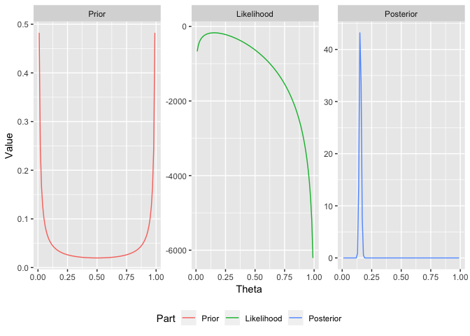
This model though is too simple, we pool all the results and assume that there is one \(\theta\) that applies to all the experiments. A better model would be to allow for variation across the experiments. Also, we thought the prior was uninformative, its actually incredibly informative at the boundaries. Can we find better values of \(\alpha _0\) and \(\beta _0\).
A Hierarchical Model
In this model, we are now assuming that each experiment has its own \(\theta _i\). Furthermore, we place a prior on \(\alpha _0\) and \(\beta _0\) we allow them to vary in the inference process aswell.
\[\begin{aligned} \theta _i \mid \alpha _0 , \beta _0 & \sim \text{Beta} (\alpha _0, \beta _0), \\ y_i \mid N_i , \theta _i & \sim \text{Binomial} (N_i, \theta _i ). \end{aligned}\]So instead of setting \(\alpha _0\) and \(\beta_0\) to specific values, we allow them to vary and find the most suitable values. But we loose the conjugacy and have to use Stan to sample from the model.
We build the model in Stan view the .stan here and sample form the posterior distribution.
stanModel <- stan_model("rats_hyper.stan")

stanData <- list()

stanData$y <- rats$y
stanData$N <- rats$N
stanData$n <- nrow(rats)

smpls <- sampling(stanModel, stanData, chains=4, iter=5000, cores=2)

plot(smpls, par=c("alpha0", "beta0"))
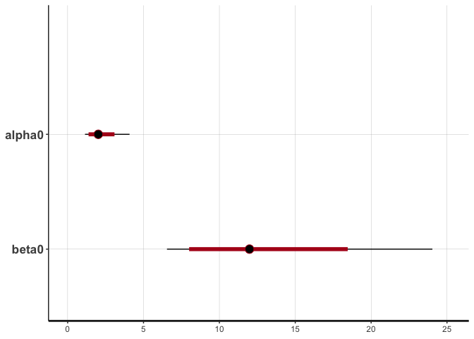
Here we can see that there is quite a bit of uncertainty around the \(\beta_0\) value. We extract the samples to use later.
as.data.frame((rstan::extract(smpls, pars=c("mu", "nu")))) -> postParams
as.data.frame((rstan::extract(smpls, pars=c("alpha0", "beta0")))) -> postParamsAlt
Dirichlet Process
What if we relaxed the assumption that the prior on \(\theta\) needs to be parametric. Instead, what if we represented our prior on \(\theta\) as an infinite mixture model, and updated it with each posterior draw.
\[\begin{aligned} \theta _i & \sim F \\ F & = \sum _{k=1} ^\infty w_k k(\theta \mid \phi _k) \end{aligned}\]where \(k\) is just the \(\text{Beta}\) distribution and \(\phi _k\) represents that distributions parameters.
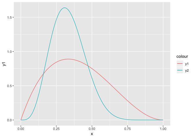
To help visualise this lets consider two components of equal weight,
wk <- c(0.5, 0.5)
phik_alpha <- c(2, 5)
phik_beta <- c(3, 10)

xGrid <- seq(0, 1, by=0.01)

frameF <- data.frame(x=xGrid,
                     y1 = wk[1] * dbeta(xGrid, phik_alpha[1], phik_beta[1]),
                     y2 = wk[2] * dbeta(xGrid, phik_alpha[2], phik_beta[2]))


ggplot(frameF) +
  geom_line(aes(x=x, y=y1, colour="y1")) +
  geom_line(aes(x=x, y=y2, colour="y2"))
Then when you combine them you get:
ggplot(frameF, aes(x=x, y=y1+y2)) + geom_line()
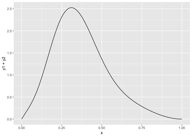
Now if we let the number of components got to infinity we can make the distribution whatever shape we want.
We want to apply the same type of logic to learn an infinite component mixture model. This means that the prior will learn the best fitting distribution.
For each iteration, we guess the prior distribution using the
PosteriorClusters function. This returns a list of weights and
parameters. We then sample from the weights for each point, to guess
what cluster it belonged too. Then using these cluster parameters we
can draw a value of \(\theta\). This is repeated for each point to
produce a new value for \(\theta _i\) for all \(i\). We then pass these
new values back into the dp object using ChangeObservations and
Fit to update the cluster parameters and weights. The process is
repeated for as many iterations as needed.
FIT <- FALSE
its <- 1500

if(FIT){

  print("Starting Fit")

  thetaDirichlet <- rbeta(nrow(rats), alphaPosterior, betaPosterior)

  dp <- DirichletProcessBeta(thetaDirichlet,
                             1,
                             mhStep = c(0.002, 0.005),
                             alphaPrior = c(2, 0.5))

  dp$numberClusters <- nrow(rats)
  dp$clusterLabels <- seq_len(nrow(rats))
  dp$clusterParameters <- PriorDraw(dp$mixingDistribution, nrow(rats))
  dp$pointsPerCluster <- rep_len(1, nrow(rats))

  dp <- Fit(dp, 1)

  postFuncEval <- matrix(ncol=its, nrow=length(xGrid))
  muPostVals <- matrix(ncol=its, nrow=nrow(rats))
  nuPostVals <- matrix(ncol=its, nrow=nrow(rats))

  pb <- txtProgressBar(max=its, width=50, char="-", style=3)

  for(i in seq_len(its)){

    postClusters <- PosteriorClusters(dp)

    postFuncEval[,i] <- PosteriorFunction(dp)(xGrid)

    wk <- sample.int(length(postClusters$weights),
                     nrow(rats),
                     replace = T,
                     prob = postClusters$weights)

    muPost <- postClusters$params[[1]][,,wk]
    nuPost <- postClusters$params[[2]][,,wk]

    aPost <- muPost * nuPost
    bPost <- (1-muPost) * nuPost

    muPostVals[,i]  <- muPost
    nuPostVals[,i]  <- nuPost

    newTheta <- rbeta(nrow(rats), aPost + rats$y, bPost + rats$N - rats$y)

    dp <- ChangeObservations(dp, newTheta)
    dp <- Fit(dp, 100, updatePrior = T, progressBar = F)

    setTxtProgressBar(pb, i)

  }

  saveList <- list()
  saveList$muPostVals <- muPostVals
  saveList$nuPostVals <- nuPostVals
  saveList$postFuncEval <- postFuncEval

  saveRDS(saveList, "dpPrior.RDS")
} else {
  print("Fit from Cache")
  saveList <- readRDS("dpPrior.RDS")
  saveList$muPostVals -> muPostVals
  saveList$nuPostVals -> nuPostVals
  saveList$postFuncEval -> postFuncEval
}
Once the fitting is finished we collect the resulting posterior samples of the prior parameters.
dirichletParamsMu <- data.frame(Value = c(muPostVals[,-(1:its/2)]))
dirichletParamsMu$Parameter= "Mu"

dirichletParamsNu <- data.frame(Value = c(nuPostVals[,-(1:its/2)]))
dirichletParamsNu$Parameter="Nu"

dirichletParams <- bind_rows(dirichletParamsMu, dirichletParamsNu)


ggplot(dirichletParams, aes(x=Value)) + geom_density() + facet_wrap(~Parameter, scales="free")

ggplot(dirichletParams, aes(x=log(Value))) + geom_density() + facet_wrap(~Parameter, scales="free")

Each peak in the density shows a cluster that is sampled in the Dirichlet process. From here we can see that there is only one real cluster for \(\mu\), but for \(\nu\) there are multiple cluster values that are sampled. It easier to see on the log scale.
nclusters <- apply(muPostVals[, -(1:its/2)], 2, function(x) length(unique(x)))
qplot(x=nclusters, geom="histogram", binwidth=1)

Here we can see that whilst the vast majority of the time it finds 1 cluster, there is plenty of samples where there is more than one cluster.
Resulting Priors
Now we compare the priors of the hierarchical model and that of the Dirichlet model.
apply(postParamsAlt, 1, function(x) dbeta(xGrid, x[1], x[2])) -> hierEval


hierEvalFrame <- data.frame(x=xGrid,
                            Mean=rowMeans(hierEval),
                            LQ = apply(hierEval, 1, quantile, probs=0.025),
                            UQ = apply(hierEval, 1, quantile, probs=1-0.025),
                            Model = "Hierarchical")

funcMean <- rowMeans(postFuncEval[,-(1:its/2)])

dirEvalFrame <- data.frame(x=xGrid,
                           Mean = rowMeans(postFuncEval),
                           LQ = apply(postFuncEval, 1, quantile, probs=0.025),
                           UQ = apply(postFuncEval, 1, quantile, probs= 1 - 0.025),
                           Model = "Dirichlet")

allEvalFrame <- bind_rows(hierEvalFrame, dirEvalFrame)

ggplot(allEvalFrame) +
  geom_ribbon(aes(x=x, ymin=LQ, ymax=UQ, colour=Model, fill=Model), alpha=0.2) +
  geom_line(aes(x=x, y=Mean, colour=Model)) +
  facet_grid(~Model) +
  scale_x_continuous(limits = c(0.01, 1-0.01)) +
  guides(colour = FALSE, fill=FALSE)

So the differences in the resulting priors are very negligible to the eye. Reassuringly, we can see that the Dirichlet model has resulted in the same shape as the hierarchical model, which in this case, suggests that our data can be modelled without the need for a non-parametric prior.
You could perform the standard model checking techniques to find out if
the Dirichlet prior performs better. I’ll leave that as an exercise for
the reader. This blog post was about showing how the dirichletprocess
package can be easily used to drop non-parametric components of models
into problems.
If you like what you see download dirichletprocess from CRAN or head
over to the Github (dirichletprocess) for the latest dev version.