Expected Goals - Overachieving or just lucky?
A new football season is on the horizon and to get the most clicks I feel like it is a good time to write a football based blogpost. Nowadays, you can’t read any transfer rumour or gossip column without someone mentioning expected goals and using it to judge whether a team, manager or player is good or bad. I’ll hopefully explain what an expected goal is and how we can use it to gain some insight on a football match.
Enjoy these types of posts? Then you should sign up for my newsletter.
There has been a steady march towards quantitative and statistical methods in football and any club worth their salt will have some sort of analytics team providing a numbers based evaluation on many different aspects of performance; be it player valuation, match analysis or tactic discussions. They will be building models and using the outputs to help make decisions.
I want to outline a basic expected goals model that we can use in two ways:
- Prematch - before a ball has even been kicked, how many goals are we expected to score?
- Postmatch - given the number of shots and other variables, how lucky or unlucky was the team with the result?
I’ll show you how a model can be used to answer these questions and will take you on the full statistical journey; obtaining the data, building the model and then using the model to answer the above questions. Later on I’ll show you a luck table and who the over and underachievers were in a COVID season.
I’ve done the analysis in R, but hopefully the steps are obvious enough to be replicated in Python or Julia, so you can still follow along even R is not your first language. There are some big code chunks that will show you all the steps to get the final graphs.
require(readr)
require(dplyr)
require(ggplot2)
require(tidyr)
require(rstanarm)
require(loo)
require(ggrepel)
require(lubridate)
require(knitr)
require(ggforce)
require(hrbrthemes)
require(wesanderson)
theme_set(theme_ipsum())
extrafont::loadfonts()
source("../BettingFunctions.R")
As always, we download the data from
https://www.football-data.co.uk. I have my own helper functions to
load the individual files in loadBulkData().
rawData <- loadBulkData()

rawData %>%
  select(Div, Season, Date,
         HomeTeam, AwayTeam,
         FTHG, FTAG,
         PSCH, PSCA, PSCD,
         HS, AS, HST, AST,
         HC, AC,
         HR, AR) %>%
  drop_na %>%
  mutate(Date = dmy(Date)) -> cleanData
We convert the odds to probabilities by taking the inverse and then normalise them to take care of the over-round. There are fancier ways of dealing with the over-round, but right now that will be overkill and for simplicity lets just use the basic method. These probabilities will feed in to the Prematch model.
cleanData %>%
  mutate(HomeProbRaw = 1/PSCH,
         AwayProbRaw = 1/PSCA,
         DrawProbRaw = 1/PSCD,
         Overround = HomeProbRaw + AwayProbRaw + DrawProbRaw,
         HomeProb = HomeProbRaw / Overround,
         AwayProb = AwayProbRaw / Overround,
         DrawProb = DrawProbRaw / Overround) -> cleanData
We now turn to separating the home and away details of each match so that each team per match is one observation. This involves just renaming the columns and adding an variable to indicate whether they are at home or not. These variables will be used in the Postmatch model.
cleanData %>%
  select(Div, Season, Date, HomeTeam, HomeProb, FTHG, HS, HST, HC, HR) %>%
  rename(Team = HomeTeam, Goals = FTHG,
         WinProb = HomeProb,
         Shots = HS, ShotsTarget = HST, Corners = HC, SendOff = HR) %>%
  mutate(Home = 1) -> homeData

cleanData %>%
  select(Div, Season, Date, AwayTeam, AwayProb, FTAG, AS, AST, AC, AR) %>%
  rename(Team = AwayTeam, Goals = FTAG,
         WinProb = AwayProb,
         Shots = AS, ShotsTarget = AST, Corners = AC, SendOff = AR) %>%
  mutate(Home = 0) -> awayData

allData <- bind_rows(homeData, awayData)

allData %>% filter(Season == "1920") -> testData
allData %>% filter(Season != "1920") -> trainData
Our test data set will be the COVID season of 1920 and all the other data will form the training data. This reduces the chance of us overfitting the model to the season we are interested in.
ggplot(allData, aes(x=Goals)) +
  geom_bar() +
  scale_x_continuous(breaks = 0:max(allData$Goals)) +
  theme_ipsum(grid="y") +
  ylab("") +
  ggtitle("Total Number of Goals")
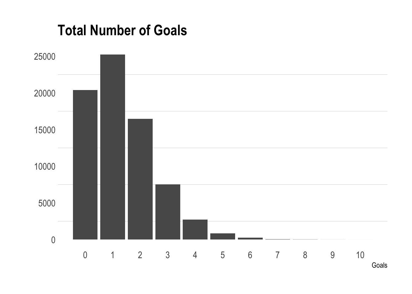
And here is a plotting showing what we are trying to predict before and after the match. For each team in a match we want to predict the number of goals they are going to score before the match and then the number of goals they should have scored given their performance in the match.
We will be using a Poisson GLM with a variety of predictors to try and model the
number of goals each team scores. Our expected goals measure will be
the resulting fitted \(\lambda\) parameter for that team in that
match. All the models will be fitten in Bayesian way using
rstanarm.
The Post Match Model
The team walks off the pitch and we want to estimate how many goals they should have scored based off a number of their statistics. For this model we will use the following:
- Number of shots
- Number of shots on target
- Number of corners
- Number of players sent off
- Whether they was at home or not
We also include a division variable to account for the different amount of goals scored in each competition.
if(file.exists("models/postMatchNull.RDS")){

  postMatchNull <- readRDS("models/postMatchNull.RDS")

} else {

  postMatchNull <- stan_glm(Goals ~ Home + Div,
                          family = "poisson", data = trainData,
                          chains = 2, cores = 2)
  saveRDS(postMatchNull, "models/postMatchNull.RDS")
}

if(file.exists("models/postMatchModel.RDS")){

  postMatchModel <- readRDS("models/postMatchModel.RDS")

} else{

  postMatchModel <- stan_glm(Goals ~ Shots + ShotsTarget + Corners + SendOff + Home + Div,
                             family = "poisson", data = trainData,
                             chains = 2, cores = 2)
  saveRDS(postMatchModel, "models/postMatchModel.RDS")

}
We fit the candidate model and a null model to give us a baseline to improve upon and then using the leave-one-out compare the models to make sure all our variables are adding some benefit to the model.
if(file.exists("models/looRes.RDS")){

  looRes <- readRDS("models/looRes.RDS")

} else {

  looRes <- compare_models(loo(postMatchNull, cores = 2),
                         loo(postMatchModel, cores = 2))
  saveRDS(looRes, "models/looRes.RDS")
}
looRes
##
## Model comparison:
## (negative 'elpd_diff' favors 1st model, positive favors 2nd)
##
## elpd_diff        se
##    9071.9     128.0
Thankfully, LOO agrees that those extra variables do help predict the number of goals and we can carry of with our analysis.
allData %>%
  mutate(PostMatchExpGoalsPred = as.numeric(exp(predict(postMatchModel, newdata = allData)))) -> allData

allData %>%
  filter(Season == "1920", Div == "E0") %>%
  group_by(Team) %>%
  summarise(PostMatchExpGoals = sum(PostMatchExpGoalsPred),
            TotalGoals = sum(Goals)) %>%
  mutate(Diff = PostMatchExpGoals - TotalGoals) %>%
  arrange(-abs(Diff)) %>%
  head(5) %>%
  kable
| Team | PostMatchExpGoals | TotalGoals | Diff |
|---|---|---|---|
| Man City | 66.61824 | 102 | -35.38176 |
| Liverpool | 57.85477 | 85 | -27.14523 |
| Tottenham | 45.35253 | 61 | -15.64747 |
| Norwich | 40.70036 | 26 | 14.70036 |
| Arsenal | 41.53747 | 56 | -14.46253 |
Here we can see an immediate weakness in the model, Man City scored almost twice as many goals as their postmatch expected goals and Liverpool scored over 25 more than their expected goals. This shows how a) there is a large amount of variance not being described by the model and b) the postmatch statistics are not enough to come up with a good reflection. But it is something, we just have to bear this in mind when we are using the model to draw any conclusions.
We could also think of this as the ‘luck factor’. Norwich according to our model would have scored 40 goals, but instead on scored 26 making them very unlucky. Whereas Man City, Liverpool, Spurs and Arsenal all outscored the model, they were ‘lucky’.
Overall, I think you can see it can be little bit of both, the model can be improved by including things like shot quality, and opponent defensive strength but there will always be some element of luck that we can quantify from the output.
The Prematch Model
Now we want to look at before the match, how many goals is a team expected to score based off the betting markets belief that they will win? For this we simply use the win probability of each team before the match. If we assume that the closing odds contains the most amount of information about a team chance of winning then there is no better predictor. If there is a better predictor, then whoever has that prediction should bet on the market, causing the odds to move and reflect that better information.
if(file.exists("models/preMatchModel.RDS")){

  preMatchModel <- readRDS("models/preMatchModel.RDS")

} else{
  preMatchModel <- stan_glm(Goals ~ WinProb, family="poisson",
                            data = as.data.frame(trainData), chains=2, cores=2)

  saveRDS(preMatchModel, "models/preMatchModel.RDS")

}

modelCheckGoals <- posterior_predict(preMatchModel,
                                     newdata = allData,
                                     draws = 1000)

allData$Prediction <- modelCheckGoals[1,]

allData %>%
  mutate(Train = if_else(Season == "1920", "Test", "Train")) %>%
  select(Goals, Prediction, Train ) %>%
  gather(Key, Goals, -Train) -> modelCheckPlot

ggplot(modelCheckPlot, aes(x=Goals, colour=Key, fill=Key)) +
  geom_bar(position="dodge") +
  facet_wrap(~Train, scales = "free_y") +
  theme(legend.position = "bottom", legend.title = element_blank()) +
  scale_color_manual(values=wes_palette("Moonrise3")) +
  scale_fill_manual(values=wes_palette("Moonrise3")) +
  theme_ipsum(grid="y") +
  theme(legend.position = "bottom", legend.title = element_blank()) +
  ylab("") +
  scale_x_continuous(breaks=0:max(modelCheckPlot$Goals))
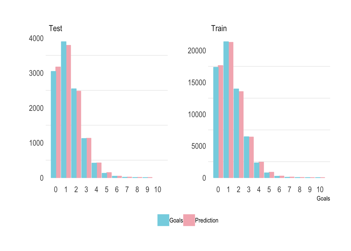
This time we want to validate the model in a slightly different way. We want to simulate the total number of goals in the test set and see how that compares to the truly observed number of goals. It all lines up nicely so our prematch model is doing the correct job.
expGoals <- posterior_linpred(preMatchModel,
                              draws = 1000,
                              transform = TRUE,
                              newdata = allData)

lqExpGoals <- apply(expGoals, 2, quantile, probs=0.05)
uqExpGoals <- apply(expGoals, 2, quantile, probs=0.95)
meanExpGoals <- apply(expGoals, 2, mean)

allData %>%
  mutate(LQ = lqExpGoals,
         UQ = uqExpGoals,
         PreMatchExpGoalsPred = meanExpGoals) -> allData

allData %>%
  filter(Season == "1920") %>%
  group_by(Div, Team) %>%
  summarise(PreMatchExpGoals = sum(PreMatchExpGoalsPred),
            PostMatchExpGoals = sum(PostMatchExpGoalsPred),
            TotalGoals = sum(Goals),
            PreMatchSpread = TotalGoals - PreMatchExpGoals,
            PostMatchSpread = TotalGoals - PostMatchExpGoals,
            N= n()) -> monthSummary

ggplot(monthSummary %>% filter(Div == "E0"),
       aes(x=PreMatchSpread, y=PostMatchSpread, label=Team)) +
  geom_point() +
  geom_vline(xintercept = 0) +
  geom_hline(yintercept = 0) +
  geom_label_repel()
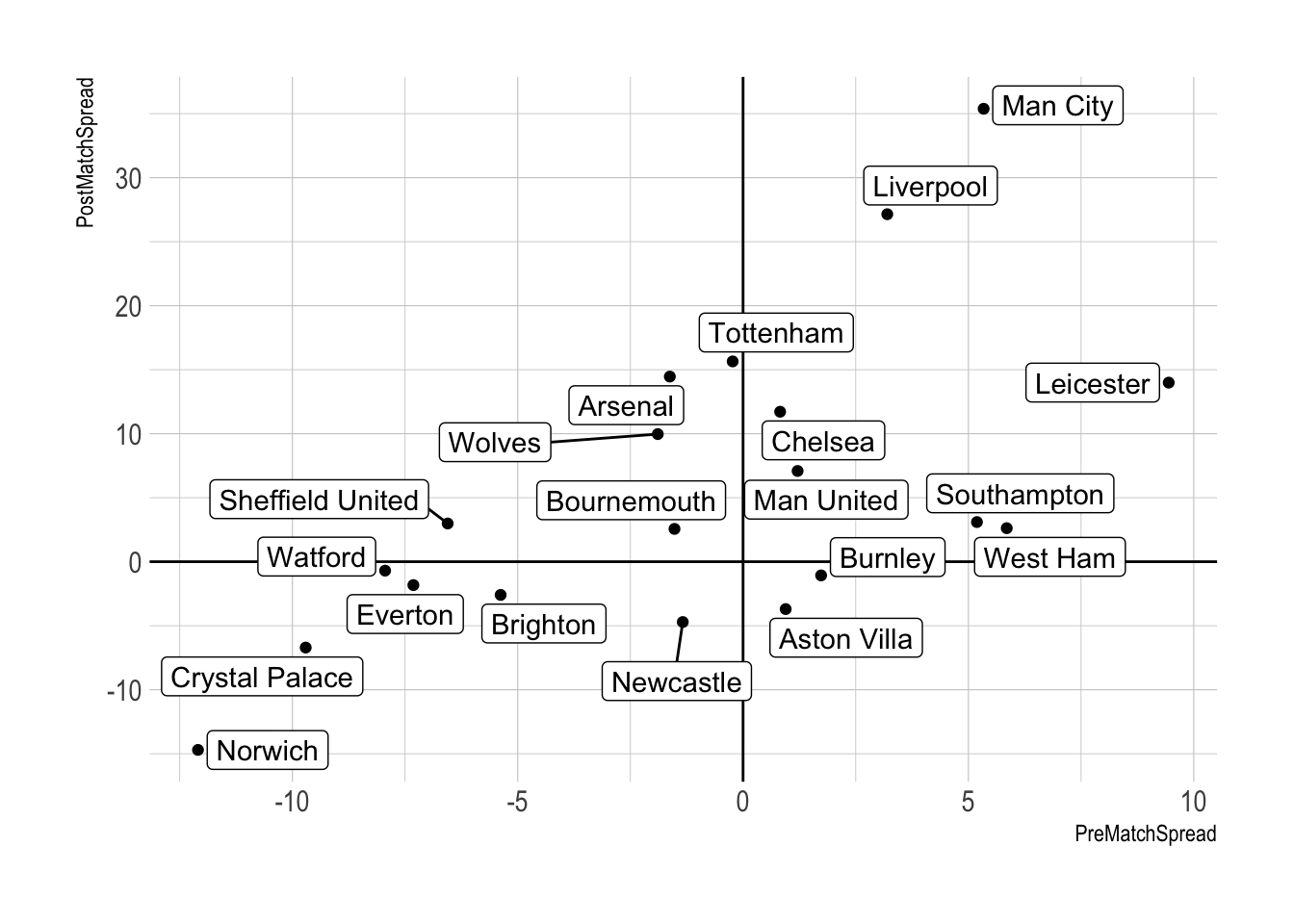
Two models, two outputs and this graph shows how we can combine the predicted goals in one graph. On the y-axis, we take the predicted number of goals from the postmatch model, subtract the number of goals actually scored on the match and take the average over the season to give a postmatch spread value. This measures luck, the number of goals they scored was greater than the suggested amount they should have got from the number of shots. On the x-axis we do the same but for the prematch model, take the predicted number of goals and subtract the actual amount they actually scored. This measures achievement and how well they done in terms of how many goals they were expected to score.
To repeat, ‘luck’ is on the y-axis, so lucky in the top half and unlucky on the bottom. Then ‘achievement’ is on the x-axis, overachievement to the right and underachievement to the left. For the Premier league its a nice visual indication of where each team ended up. Leicester are the standout, lucky and overachieving and even Man City was luckier than Liverpool but obviously not where it counted. In the bad zone you’ve got Norwich and Watford being both underachieving and unlucky.
A Prediction for Next Season
So can we use this model to base some predictions for next season? Potentially you think that the unlucky teams will have a turn of fortune in the new season, or that promoted teams got promoted by luck rather than skill.
promoted <- c("Leeds", "West Brom", "Fulham",
              "Coventry", "Rotherham", "Wycombe",
              "Swindon", "Crewe", "Plymouth")

relegated <- c("Bournemouth", "Watford", "Norwich",
               "Charlton", "Wigan", "Hull",
               "Tranmere", "Southend", "Bolton",
               "Stevenage")

monthSummary %>%
  mutate(Result = case_when(Team %in% promoted ~ "Promoted",
                            Team %in% relegated ~ "Relegated",
                            TRUE ~ "Other")) -> monthSummary

ggplot(monthSummary %>%
         filter(Result %in% c("Promoted", "Relegated")),
       aes(x = PreMatchSpread/N, y = PostMatchSpread/N, label=Team, colour=Result)) +
  geom_vline(xintercept = 0) +
  geom_hline(yintercept = 0) +
  xlab("Pre Match Spread") +
  ylab("Post Match Spread") +
  geom_circle(aes(r=0.25, x0=0, y0=0), inherit.aes = FALSE)+
  geom_circle(aes(r=0.5, x0=0, y0=0), inherit.aes = FALSE)+
  geom_point() +
  geom_label_repel(show.legend = FALSE) +
  theme(legend.position = "bottom", legend.title = element_blank()) +
  scale_colour_manual(values=rev(wes_palette("Darjeeling1", n=2)))
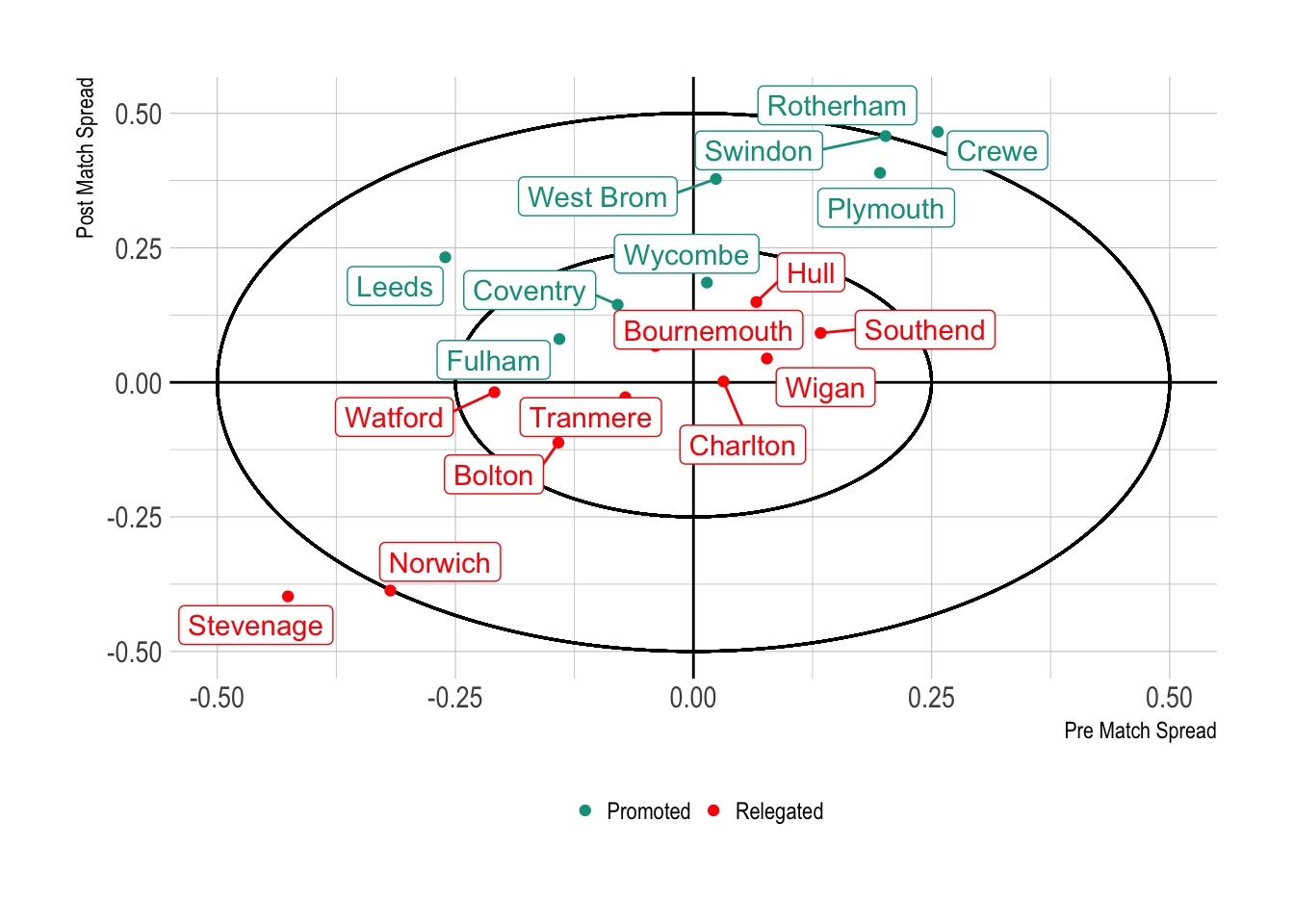
As the number of games between the leagues is different we now need to divide by the total matches played to get an average over/under performance. We add two circles at 0.25 and 0.5 goals over/under the actual goals scored to help keep contextualise the values.
Here we can see a partial split between the promoted and relegated teams from this season. You have the likes of Stevenage and Norwich that continuously underperformed, whereas Hull and Southend outperformed (Southend have their own issues though, so in this case it looks like they were always certain to be relegated).
Let’s focus on the extremes; Stevenage and Norwich had horrendous seasons and thus we can suspect that they won’t get promoted straight away. Likewise for Rotherham and Crewe, they out performed the models so well, that they should regress to the mean next season and potentially get relegated. It’s all a bit handy-wavy though, so lets see where the odds are now and then track them through the season.
Promoted:
- Hull - Buy at 4.5 (William Hill)
Not relegated:
- Leeds - Sell at 5.4 (Smarkets)
- Coventry - Sell at 7.2 (Smarkets)
Relegated:
- Rotherham - Buy at 3.5 (William Hill)
- Crewe - Buy at 5.0 (Sky Bet)
Each month I’ll update the prices and see how well the strategy pays off.
Conclusion
So there we go, using publicly available data we’ve got a postmatch and a prematch model. Prematch uses the match probabilities to make a guess at the number of goals a team will score which can then be used to quantify which teams over and underachieved. Postmatch uses the amount of shots, shots on target, corners and sent off players to come up with how lucky a team was. We’ve then used these models to come up with the predictions for the next season and will track the prices to see how good of a prediction they actually are.
This type of analysis is a good stepping stone for anyone interested in building their own expected goals model. Mine is pretty much as basic as it gets but there is all sorts of scope to include some lag effects, rolling averages and to just generally develop the model further.
So overall, what is an expected goal? It’s just the predicted amount of goals that we obtain from some model. Done.
Notes
- Graph themes are from
hrbrthemes - Colours themes are from
wesanderson