Getting Started with High Frequency Finance using Crypto Data and Julia
Crypto is making finance democratic. My PhD was originally going to be on the limit order book and modeling events that can change its state. However, I just couldn’t get the data. Now, anyone can access different exchanges limit orders books with simple API calls. My Julia package CoinbasePro.jl does exactly that and you can get full market data without even having to sign up.
Sure, crypto markets will be less liquid and more erratic than your traditional datasets, but you get what you pay for. So if you are a student looking to get stuck into high frequency or quant finance, this type of data is exactly what you are looking for.
Enjoy these types of posts? Then you should sign up for my newsletter.
This blog post will introduce you to different concepts:
To access all this free data I’ve written an interface to the CoinbasePro API in Julia. It’s in the general repo and you can install it the normal way or take a look at the code here:
using Plots, Statistics, StatsBase, DataFrames, DataFramesMeta
using CoinbasePro
The Limit Order Book
The limit order book (LOB) is the collection of orders at which people are willing to buy and sell something. Rather than sending a market order to trade at whatever price, you can send an order into the book and it will execute if the price ever reaches your order.
When it comes to order book data, it gets categorised into three different types.
- Level 1: The best price to buy or sell at. AKA the “top level” of the book.
- Level 2: Aggregated levels, 50 levels at which people are willing to buy and sell.
- Level 3: The full order book
With the book function you chose what level and currency pair to pull from Coinbase.
l1 = CoinbasePro.book("btc-usd", 1)
first(l1, 5)
| num-orders_ask | price_ask | size_ask | num-orders_bid | price_bid | size_bid | |
|---|---|---|---|---|---|---|
| Int64 | Float64 | Float64 | Int64 | Float64 | Float64 | |
| 1 | 3 | 36308.2 | 0.0350698 | 1 | 36308.2 | 0.214675 |
Just one row, the top level, if you were to place a market order of a size less than the size above, this is the price you would be filled at. If your trade size was larger than the listed price, you would also consume the next levels until your full size was complete.
bookData = CoinbasePro.book("btc-usd", 2)
first(bookData, 5)
| num-orders_ask | price_ask | size_ask | num-orders_bid | price_bid | size_bid | |
|---|---|---|---|---|---|---|
| Int64 | Float64 | Float64 | Int64 | Float64 | Float64 | |
| 1 | 3 | 36313.6 | 0.350958 | 2 | 36313.6 | 0.0761817 |
| 2 | 1 | 36313.6 | 0.0221 | 2 | 36313.0 | 2.07568 |
| 3 | 1 | 36313.9 | 0.0441907 | 1 | 36313.0 | 0.0195784 |
| 4 | 2 | 36315.0 | 0.400577 | 1 | 36312.4 | 0.137662 |
| 5 | 1 | 36324.1 | 0.0542957 | 1 | 36312.4 | 2.42316 |
Here is the top 50 levels at which people will buy and sell at at the given time we called the function. Can now get a better idea of where people will buy and sell. As it is aggregated, there might be multiple orders at one price rather than just a single large order.
l3 = CoinbasePro.book("btc-usd", 3)
first(l3, 5)
| price_ask | size_ask | level | |
|---|---|---|---|
| Float64 | Float64 | Int64 | |
| 1 | 36313.6 | 0.319169 | 1 |
| 2 | 36313.6 | 0.009689 | 2 |
| 3 | 36313.6 | 0.0221 | 3 |
| 4 | 36313.6 | 0.0221 | 4 |
| 5 | 36313.9 | 0.0441907 | 5 |
Finally the full order book, this gives every order currently available. So with each increasing level we get more and more detail about what the state of the market is. In the 3rd level there are over 50,000 different orders available.
nrow(l3)
55865
High frequency trading is all about knowing where and when to place orders and at what size. If you think you can predict where the price will be in the next second (or even shorter timescales) you can buy now, place a limit order where you think the price will go and hope it moves in that direction. Likewise, if you suddenly start observing lots of cancellations at particular levels, that might also give some information at what is happening to the market.
The good thing about the Coinbase API is you can now start to get a feel for how to manage this type of data free and easily.
Sweeping the Book
How can we use the information from the order book? What is the average price if we traded at every level? If we need to trade a large amount, we would go through each layer of the order book, trading at that price and eating up liquidity. But that comes at a price, our overall average price will be worse than the best price when we started. How much worse depends on the overal amount of liquidity available at a given time. So being on top of how much it would cost to trade a large amount at a given time is key for risk management.
To calculate this using the order book data we simply add up the amount at each level and the cumulative average price at each level. We do this calculation on both the bid and ask side to see how they differ.
askSize = cumsum(bookData[!, "size_ask"])
askCost = map(n -> sum(bookData[!, "size_ask"][1:n] .* bookData[!, "price_ask"][1:n]) / askSize[n], 1:nrow(bookData))

bidSize = cumsum(bookData[!, "size_bid"])
bidCost = map(n -> sum(bookData[!, "size_bid"][1:n] .* bookData[!, "price_bid"][1:n]) / bidSize[n], 1:nrow(bookData));
We can now plot the total amount on the x axis and the total cost on the y axis.
plot(askSize, 1e4 .* ((askCost ./ bookData[!, "price_ask"][1]) .- 1), label="Ask", xlabel="Number of Bitcoins", ylabel="Cost (bps)")
plot!(bidSize, abs.(1e4 .* ((bidCost ./ bookData[!, "price_bid"][1]) .- 1)), label="Bid")

Only issue here, is the x axis is in Bitcoin’s and not the easiest to interpret. The y axis is in basis points (bps) which is a percentage of the total traded amount. 1bps = 0.01%. So we want to convert both axis into dollars so you can understand it all a bit easier. For this we will need the midprice of BTC-USD, which we get using the ticker function from the CoinbasePro API.
tickerStats = CoinbasePro.ticker("BTC-USD")
| ask | bid | price | size | time | volume | |
|---|---|---|---|---|---|---|
| Float64 | Float64 | Float64 | Float64 | Int64 | Float64 | |
| 1 | 36339.7 | 36338.5 | 36339.6 | 0.00543844 | 2021-06-10T21:09:18.260533Z | 20600.9 |
mid = (tickerStats.ask + tickerStats.bid)/2
1-element Vector{Float64}:
 36339.11
This gives a quick summary of the currency which we can then convert our previous calculation into dollars.
askBps = 1e4 .* ((askCost ./ bookData[!, "price_ask"][1]) .- 1)
bidBps = abs.(1e4 .* ((bidCost ./ bookData[!, "price_bid"][1]) .- 1))

plot(askSize .* mid /1e6, (askBps /1e4) .* askSize .* mid, label="Ask", xlabel="Million of Dollars")
plot!(bidSize .* mid /1e6, (bidBps/1e4) .* bidSize .* mid, label="Bid", ylabel = "Cost (dollars)")

Now we can interpret this chart a little easier. If we were to buy 500k USD worth of bitcoin we need to look at the ask curve. We can see that this roughly intercepts the y-axis as around 50$, which means we will pay $50 dollars to get our 500k order executed at current liquidity levels.
Now this isn’t a “direct” cost, like commission or a fee for trading, it is an execution cost.
- You decide to buy 500k worth of BTC.
- You send the market order to the exchange and it executes eating through all the levels.
- When the Bitcoin is in your wallet, you’ve actually only got 499,950 worth.
- This missing $50 can be attributed to execution costs.
You pay these execution costs because you are eating through liquidity.
Now minimising these costs is an entire industry and ultimately what a trader gets paid to do.
Last 1000 Trades
Coinbase also let you obtain the last 1000 trades, which can provide all sorts of insights. Echoing the introduction, you would never get this kind of information for free for any other asset classes.
trades, pages = CoinbasePro.trades("BTC-USD")
first(trades, 5)
| price | side | size | time | trade_id | |
|---|---|---|---|---|---|
| Float64 | String | Float64 | DateTim… | Int64 | |
| 1 | 36338.5 | sell | 0.0269793 | 2021-06-10T21:09:22.105 | 185030310 |
| 2 | 36338.5 | buy | 0.0191325 | 2021-06-10T21:09:21.888 | 185030309 |
| 3 | 36338.5 | buy | 0.045 | 2021-06-10T21:09:21.888 | 185030308 |
| 4 | 36338.5 | buy | 0.000999 | 2021-06-10T21:09:21.888 | 185030307 |
| 5 | 36338.5 | buy | 0.000701 | 2021-06-10T21:09:21.521 | 185030306 |
plot(trades.time, trades.price, group=trades.side, seriestype=:scatter, xlabel="Time", ylabel="Price")

Here you can see buys and sells happening in flurries over a very short period of time.
trades_g = groupby(trades, :side)
@combine(trades_g, AvgPrice = mean(:price),
                   N = length(:price),
                   TotalNotional = sum(:size),
                   AvgWPrice = mean(:price, Weights(:size)))
| side | AvgPrice | N | TotalNotional | AvgWPrice | |
|---|---|---|---|---|---|
| String | Float64 | Int64 | Float64 | Float64 | |
| 1 | sell | 36351.6 | 643 | 14.6543 | 36358.4 |
| 2 | buy | 36344.6 | 357 | 19.2213 | 36328.8 |
More sellers than buyers, hence the price over the last 1000 trades has moved down. Supply and demand!
Price Impact
Using the trades we can build up a (very) simple model of price impact. Price impact is how much you move the market by trading. With each trade we look at the absolute price difference of the next traded price. But first we have to aggregate trades that happen as the same time and in the same direction.
sort!(trades, :time)

gtrades = groupby(trades, [:time, :side])
tradeS = @combine(gtrades, AvgPrice = mean(:price, Weights(:size)),
                           TotalSize = sum(:size),
                           N = length(:price))


plot(log.(tradeS[2:end, :TotalSize] .+ 1), abs.(diff(log.(tradeS.AvgPrice))), seriestype=:scatter, label=:none, xlabel="Trade Size", ylabel="Impact")

Here we can see that it is very noisy and difficult to pull out any real trend. 1000 trades isn’t really enough to build this type of model, and also my approach of taking the price of the next trade could be improved too. But I’ll leave that as an exercise to the reader.
tradeS.Impact = [NaN; diff(log.(tradeS.AvgPrice))]
tradeS.Sign = [x == "sell" ? -1 : 1 for x in tradeS.side]
tradeS.SignedImpact = tradeS.Impact .* tradeS.Sign
first(tradeS, 5)
| time | side | AvgPrice | TotalSize | N | Impact | Sign | |
|---|---|---|---|---|---|---|---|
| DateTim… | String | Float64 | Float64 | Int64 | Float64 | Int64 | |
| 1 | 2021-06-10T21:04:53.286 | sell | 36378.0 | 0.0394498 | 2 | NaN | -1 |
| 2 | 2021-06-10T21:04:53.658 | sell | 36378.0 | 0.00054482 | 1 | 0.0 | -1 |
| 3 | 2021-06-10T21:04:54.461 | sell | 36378.0 | 0.00404794 | 1 | 0.0 | -1 |
| 4 | 2021-06-10T21:04:54.505 | sell | 36378.0 | 0.00103966 | 1 | 0.0 | -1 |
| 5 | 2021-06-10T21:04:56.307 | buy | 36378.0 | 3.177e-5 | 1 | -2.74891e-7 | 1 |
using CategoricalArrays

tradeS = tradeS[2:end, :]

tradeS.SizeBucket = cut(tradeS.TotalSize, quantile(tradeS.TotalSize, 0:0.1:1), extend=true)
tradeSG = groupby(tradeS, [:SizeBucket, :side])
quantileSummary = @combine(tradeSG, AvgSize = mean(:TotalSize), MeanImpact = mean(:Impact), MeanAbsImpact = mean(abs.(:Impact)))

plot(log.(quantileSummary.AvgSize), log.(quantileSummary.MeanAbsImpact), group=quantileSummary.side, seriestype=:scatter)

By looking at the quantiles of the trade size and looking at buys and sells separately this perhaps a bit more of a relationship, but again, nothing conclusive. I suggest that you collect more data and read some of papers on market impact. A good place to start would be these two:
Trade Sign Correlation
The distribution of trade signs also gives insight into the nature of markets. The notion of ‘long memory’ in markets can be attributed to the slicing up of a large order. As we have shown in the above section, each trade eats up liquidity and you pay a price for that, if you can break up an order into smaller chunks such that the sum of the costs of each small order is less than that if you would have made a big order, well thats more money in your pocket.
There are also lots of other reasons for splitting up a large order, suddenly flooding the market with a big trade size will cause an adverse reaction in the price and in essence ‘reveal’ how you are positioned. So being able to split an order is a necessity.
A great paper that looks at both order sign dynamics and also trade size distribution (which we will come onto later) can be found here: https://arxiv.org/pdf/cond-mat/0412708.pdf . I’ve largely take what they do and applied it to the crypto data from Coinbase.
First we aggregate those trades that occurred on the same timestamp and in the same direction.
aggTrades = @combine(gtrades, N=length(:size), TotalSize = sum(:size))
first(aggTrades, 5)
| time | side | N | TotalSize | |
|---|---|---|---|---|
| DateTim… | String | Int64 | Float64 | |
| 1 | 2021-06-10T21:04:53.286 | sell | 2 | 0.0394498 |
| 2 | 2021-06-10T21:04:53.658 | sell | 1 | 0.00054482 |
| 3 | 2021-06-10T21:04:54.461 | sell | 1 | 0.00404794 |
| 4 | 2021-06-10T21:04:54.505 | sell | 1 | 0.00103966 |
| 5 | 2021-06-10T21:04:56.307 | buy | 1 | 3.177e-5 |
For each of the aggregated timestamp trades we assign buys as 1 and sells as -1. Then by looking at the autocorrelation between the trades we can come up with an explanation of how likely a buy is followed by another buy.
sides = aggTrades.side
sidesI = zeros(length(sides))
sidesI[sides .== "buy"] .= 1
sidesI[sides .== "sell"] .= -1

ac = autocor(sidesI);
As we are looking at a possible power law relationship, we take the log of both the autocorrelation and the lag to see if there is a straight line. Which there appears to be.
lags = eachindex(ac)
posInds = findall(ac .> 0)

acPlot = plot(lags, ac, seriestype=:scatter, label=:none, xlabel="Lag", ylabel="Correlation")
acLogPlot = plot(log.(lags[posInds]), log.(ac[posInds]), seriestype=:scatter, label=:none, xlabel = "log(Lag)", ylabel="log(Correlation)")
plot(acPlot, acLogPlot)

We can simply model the relationship like they do in the paper: \(\tau ^ \gamma\)
where \(\tau\) is the lag. We also remove some of the outliers to stop them influencing the result.
using GLM
modelFrame = DataFrame(LogAC = log.(ac[posInds]), LogLag = log.(lags[posInds]))

m = lm(@formula(LogAC ~ LogLag), modelFrame)
StatsModels.TableRegressionModel{LinearModel{GLM.LmResp{Vector{Float64}}, GLM.DensePredChol{Float64, LinearAlgebra.CholeskyPivoted{Float64, Matrix{Float64}}}}, Matrix{Float64}}

LogAC ~ 1 + LogLag

Coefficients:
─────────────────────────────────────────────────────────────────────────
                 Coef.  Std. Error      t  Pr(>|t|)  Lower 95%  Upper 95%
─────────────────────────────────────────────────────────────────────────
(Intercept)  -2.22219     0.642869  -3.46    0.0032  -3.58501   -0.85937
LogLag       -0.407497    0.275649  -1.48    0.1587  -0.991846   0.176853
─────────────────────────────────────────────────────────────────────────
plot!(acLogPlot, log.(0:30), coef(m)[1] .+ coef(m)[2] .* log.(0:30), label="Power Law", xlabel = "log(Lag)", ylabel="log(Correlation)")

We can see the log model fits well and we arrive at a \(\gamma\) value of around -0.4 which seems sensible and comparable to their value of -0.57 for some stocks. The paper uses a lot more data than just the 1000 trades we have access to aswell, but again, you can collect more data and see how the relationship evolves or changes across different pairs.
Trade Size Distribution
There is also a significant amount of work that is concerned with the distribution of each trade size observed. We calculate the empirical distribution and plot that on both a linear and log scale. Again, this is covered in the above paper.
sizes = aggTrades.TotalSize
uSizes = unique(aggTrades.TotalSize)

empF = ecdf(sizes)

tradesSizePlot = plot((uSizes), (1 .- empF(uSizes)), seriestype=:scatter, label="P(V > x)", xlabel="Trade Size", ylabel="Probability")
tradesSizeLogPlot = plot(log.(uSizes), log.(1 .- empF(uSizes)), seriestype=:scatter, label="P(V > x)", xlabel = "log(Trade Size)", ylabel="log(Probability)")

plot(tradesSizePlot, tradesSizeLogPlot)

The log-log plot indicates that there is some power law behaviour in the tail of the distribution. Estimating this power lower can be achieved in a number of ways, but like the above paper, I’ll use the Hill estimator to calculate the tail parameter. This is a different method as to how we estimated the above power law and comes from the theory of extreme values. I’ve copied the form of the estimator from the R package ptsuite and you can find the Hill estimator equation.
In short, it is a method for estimating the tail of a distribution when there are heavy tails. I think I’m going to write a separate blog post on this type of estimation, as it is interesting in its own right. But for now, take this equation as how we will come up with an \(\alpha\) value.
function hill_estimator(sizes, k)
    sizes_sort = sort(sizes)
    N = length(sizes_sort)
    res = log.(sizes_sort[(N-k+1):N] / sizes_sort[N-k])
    k*(1/sum(res))
end
hill_estimator (generic function with 1 method)
For this estimator we need to chose a threshold \(k\) and take all the values above that to calculate the parameter.
alphak = [hill_estimator(sizes, k) for k in 1:(length(sizes)-1)]
plot(1:(length(sizes)-1), alphak, seriestype= :scatter, xlabel="k", ylabel="Alpha", label=:none)

last(alphak, 5)
5-element Vector{Float64}:
 0.229504703150391
 0.22575089901110806
 0.2080699145436874
 0.1867189489090256
 0.1457502984372589
We could say that the value is converging to a value of around 0.2, but I don’t think we can trust that too much. It looks like a lack of data to really come up with a good estimate, 1000 trades at the end of the day isn’t enough. Again, in the paper, they calculate a value of a value -1.59, so quite a bit of difference to the crypto data. Buy again, this is a much smaller dataset compared to the papers stock data.
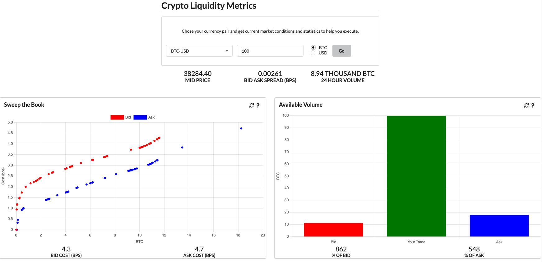
Crypto Liquidity Metrics
Now after writing all this and going through the calculations I decided to learn some javascript and replicate some of the graphs here in a website. I’ve called it https://cryptoliquiditymetrics.com/ and it connects to the same Coinbase API to produce some insight into the current state of different cryptocurrencies at a given time. Check it out and hopefully it gives you a bit of market intelligence.
Conclusion
Hopefully you’ve now got a good idea about the basic approaches to high frequency finance and different models that are used to describe the price dynamics. I am only scratching the surface though and there is so much more out there that can be easily applied using the data from the CoinbasePro.jl module.
As I kept saying, getting 1000 trades at a time is a bit limiting, so I will be on the hunt for a larger data set of crypto trade data.
If there is anything you want me to specifically look at, let me know in the comments below!
- Julia 1.6
- CoinbasePro.jl 0.1.1