Custom Mixtures with the dirichletprocess R package
In my previous article I showed how you can use the dirichletprocess package for non-parametric density estimation. This time I will demonstrate how you can use the package to create your own mixture models. The ease of creating your own mixture models is the main advantage of our dirichletprocess package compared to the others out there. By using the S3 class system in R, you can easily build your own Dirichlet process mixture of what ever distribution you want.
Firstly, make sure you have downloaded the package from CRAN.
#install.packages("dirichletprocess")
library(dirichletprocess)
library(ggplot2)
A Dirichlet process object relies on its mixingDistribution object to carry out the necessary steps for inference. If we look at one of the default mixture models available we can see that a mixingDistribution object is easy to interpret.
dp <- DirichletProcessGaussian(rnorm(10))
dp$mixingDistribution
## $distribution
## [1] "normal"
##
## $priorParameters
## [1] 0 1 1 1
##
## $conjugate
## [1] "conjugate"
##
## $mhStepSize
## NULL
##
## $hyperPriorParameters
## NULL
##
## attr(,"class")
## [1] "list"      "normal"    "conjugate"
The mixingDistribtuion inside the dp object has a number of fields. The name of the distribution, the prior parameters for the prior distribution and whether it is conjugate (with extra fields if it is non-conjugate). As a new conjugate mixture model is slightly easier to create we will start with that. The name of the distribution is then used to look up the other functions for performing the sampling. Therefore, what ever you pass into the distribution field is used to find the new custom functions.
A New Conjugate Mixture Model
The user must decide what distribution they wish to mix. In this example we will use a mixture of exponential distributions as our example. The unknown parameter that we will be sampling is \(\theta \). For a prior distribution we will be using the gamma distribution, which has two parameters \(\alpha _0 , \beta _0 \). We also pass these values into the constructor function.
We use the constructor function to build a new mixingDistribution object that will be used by the Dirichlet process functions.
expMd <- MixingDistribution(distribution = "exp", priorParameters = c(0.1,0.1), conjugate = "conjugate")
As we have used “exp” in the distribution field of our new mixing distribution object, all the subsequent functions that we create must be suffixed with .exp so that R can apply the correct functions.
All mixing distribution objects need a Likelihood function. This returns the pdf of the distribution for some data x and parameter theta.
Likelihood.exp <- function(mdobj, x, theta){
  as.numeric(dexp(x, theta[[1]]))
}
Now we need to define the prior distribution function for the parameter theta. As the exponential distribution has a conjugate prior of the gamma distribution we shall use that,
The gamma distribution has two parameters that will be stored in the mixingDistribution object.
PriorDraw.exp <- function(mdobj, n){
  draws <- rgamma(n, mdobj$priorParameters[1], mdobj$priorParameters[2])
  theta <- list(array(draws, dim=c(1,1,n)))
  return(theta)
}
The prior is conjugate so we can write a closed form of the posterior distribution
\[\theta \mid x_1, \ldots, x_n \sim \text{Gamma} (\alpha _0 + n, \beta _0 + \sum _i ^n x).\]Of course, easily translated to R code.
PosteriorDraw.exp <- function(mdobj, x, n=1){
  priorParameters <- mdobj$priorParameters
  theta <- rgamma(n, priorParameters[1] + length(x), priorParameters[2] + sum(x))
  return(list(array(theta, dim=c(1,1,n))))
}
Now the trickiest part of writing a new conjugate mixture is the predictive function. This is the marginal distribution of the data
\[\begin{aligned} p(x) & = \int _\theta p(x, \theta), \\ & = \int p(x \mid \theta) p(\theta) \mathrm{d} \theta . \end{aligned}\]Which evaluates to the ratio between the normalisation constants of the prior distribution and the posterior distribution. We want to calculate this predictive for each data point \(x_i\).
Predictive.exp <- function(mdobj, x){

  priorParameters <- mdobj$priorParameters

  pred <- numeric(length(x))

  for(i in seq_along(x)){
    alphaPost <- priorParameters[1] + length(x[i])
    betaPost <- priorParameters[2] + sum(x[i])
    pred[i] <- (gamma(alphaPost)/gamma(priorParameters[1])) * ((priorParameters[2] ^priorParameters[1])/(betaPost^alphaPost))
  }
  return(pred)
}
Now, with our functions defined and our new object created, we can use DirichletProcessCreate to build our new object. We use some synthetic data to make sure everything is working fine.
yTest <- c(rexp(100, 10), rexp(100, 0.1))

dp <- DirichletProcessCreate(yTest, expMd)
dp <- Initialise(dp)
dp <- Fit(dp, 1000, progressBar = FALSE)
data.frame(Weight=dp$weights, Theta=unlist(c(dp$clusterParameters)))
| Weight | Theta |
|---|---|
| 0.49 | 0.09084329 |
| 0.51 | 8.73310009 |
Here we can see that the correct weights are found with parameters close to their true values.
We can also plot the results to see how well our process has worked.
xGrid <- seq(0, 1, by=0.01)

postEval <- replicate(100, PosteriorFunction(dp)(xGrid))

meanFrame <- data.frame(Mean=rowMeans(postEval), x=xGrid)
quantileFrame <- data.frame(x=xGrid, t(apply(postEval, 1, quantile, prob=c(0.03, 0.97))))
trueFrame <- data.frame(x=xGrid, y=(0.5*dexp(xGrid, 10)+0.5*dexp(xGrid, 0.1)))

ggplot()  + geom_ribbon(data=quantileFrame, aes(x=x, ymin=X3., ymax=X97.), alpha=0.4) + geom_line(data=meanFrame, aes(x=x, y=Mean, colour="Posterior Mean")) + geom_line(data=trueFrame, aes(x=x, y=y, colour="True"))

Here we can see that the true generating function has been recovered nicely.
Sunspots
In R there is a dataset called sunspots. This consists of the average number of sunspots from 1749 to 1983. A sunspot is where a small part of the sun appears darker due to changes in the magnetic field of the sun. We are interested in modelling the overall distribution of these measurements. We shall be using our newly created Dirichlet process mixture of exponentials.
dp <- DirichletProcessCreate(c(sunspots), expMd)
dp <- Initialise(dp)
dp <- Fit(dp, 1000, progressBar = FALSE)
To look at the number of cluster in the data, we can just calculated the length of the weight vector after each iteration.
numClusters <- sapply(dp$weightsChain, length)
qplot(x=numClusters, geom="histogram", binwidth=1)

It looks like there is definitely two clusters in the data.
Now if we plot the posterior samples of the function, we can see how it compares to the true distribution.
xGrid <- seq(0, 250, by=0.1)
postSamps <- data.frame(lapply(750:1000, function(i) PosteriorFunction(dp, i)(xGrid)))

meanFrame <- data.frame(Mean=rowMeans(postSamps), x=xGrid)
quantileFrame <- data.frame(x=xGrid, t(apply(postSamps, 1, quantile, prob=c(0.03, 0.97))))

ggplot() + geom_histogram(data=data.frame(x=c(sunspots)), fill="cornflowerblue", aes(x=x, y=..density..), binwidth = 10) + geom_ribbon(data=quantileFrame, aes(x=x, ymin=X3., ymax=X97.), alpha=0.6) + geom_line(data=meanFrame, aes(x=x,y=Mean, colour="Posterior Mean")) + coord_cartesian(ylim = c(0,0.015))
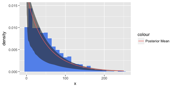
Now this is probably not the greatest model for the data. Most of the bins fall outside of the credible interval. But it is an interesting application of a Dirichlet mixture model and highlights how easy it is to create your own mixture distribution using our dirichletprocess package.