Density Estimation with the dirichletprocesss R package
With the release of the dirichletprocess package I will be writing a series of tutorials on how to use Dirichlet processes for nonparameteric Bayesian statistics. In this first tutorial we will be using a Dirichlet process for density estimation.
What is a Dirichlet process?
Reading the Wikipedia article on Dirichlet processes isn’t all that helpful for building a picture of what a Dirichlet process is and how it can be used in statistics. So here is my attempt at high level explanation!
Lets assume we have some data \(\mathbf{y}\) that is from some distribution \(F\). Now \(F\) can be any kind of weird and wonderful shape. It can be bimodal or even multimodal. It could be fully bounded or strictly positive. Basically, we are not limited to your normal parametric distributions such as Normal, Gamma etc. Instead, we are going to use a Dirichlet process to approximate \(F\) by assuming is a mixture of some parametric distribution \(K(\theta)\) where \(\theta\) are the parameters of this parametric distribution.
Now your data is made up of individual observations \(y_i\) and you chose a building block distribution \(K\) that we will combine to form \(F\). Each of these observations is from its own distribution \(K(\theta _i)\) with its own parameter \(\theta _i\). So if you have 20 data points, you will have 20 \(\theta_i\)’s. But here is the key point of a Dirichlet process: Some of these \(\theta _i\)’s will be the same as each other. So at the end you will hopefully have a smaller set of unique \(\theta _i\)’s across your data. Whilst each datapoint has its own parameter, it is not necessarily a unique parameter.
To fit a Dirichlet process, you iterate through all the datapoints, checking whether a datapoint \(y_i\) should be assigned a parameter from the other \(\theta _j\)’s assigned to \(y_j\), or whether a new \(\theta _i\) should be used. Eventually, you will find a point where every data point has its best parameter assigned and no more changes happen and you have fit your Dirichlet process to the data.
Modeling Time!
Now lets take that explanation and apply it to some data. The
faithful data set looks contains two columns, one indicating the
waiting time between eruptions of the Old Faithful geyser and another
indicating the length of eruptions.
head(faithful)| eruptions | waiting | |
|---|---|---|
| 1 | 3.600 | 79 |
| 2 | 1.800 | 54 |
| 3 | 3.333 | 74 |
| 4 | 2.283 | 62 |
| 5 | 4.533 | 85 |
| 6 | 2.883 | 55 |
We are interested in the distribution of the waiting times between eruptions. When we look at a histogram of the waiting times we find that the data is bimodal.
ggplot(faithful, aes(x=waiting)) + geom_histogram(binwidth = 1)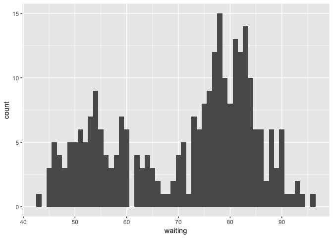
How could we model this in a Bayesian way and arrive at a probability distribution for this data? The answer: a Dirichlet process.
We believe that the waiting data is from a mixture of Normal distributions with parameters \(\theta_i = \{ \mu _i , \sigma _i \}\). So from our previous explanation, our \(K\) is the normal distribution, and each data point will have its own mean and variance. But remember, these parameters are not unique, multiple data points can have the same parameters. This means we expect the parameters to converge to a number of select clusters which will accurately model the data.
Now for the dirichletprocess bit.
Before we begin, make sure you install and load the package.
install.packages('dirichletprocess')
library(dirichletprocess)
Now we want to transform our data so that it is zero mean and unit variance. Always a good idea for any machine learning problem.
faithfulTrans <- (faithful$waiting - mean(faithful$waiting))/sd(faithful$waiting)Now we want to create our dirichletprocess object. As it is a mixture of Normal distributions, we want to use the DirichletProcessGaussian function.
dp <- DirichletProcessGaussian(faithfulTrans)We are now ready to fit our object. In future tutorials I will show how you can modify certain properties of the dp object to change how the object is initialised.
As this is a Bayesian method, we now wish to sample from the posterior distribution. To do this, we use the Fit function on the dp object and specify how many iterations we wish to run for. In this case 1000 will be plenty.
dp <- Fit(dp, 1000)Now our package has done all the heavy lifting and we have arrived at an object with our parameter samples. We can simply plot the dp object and see the resulting density is has found.
plot(dp)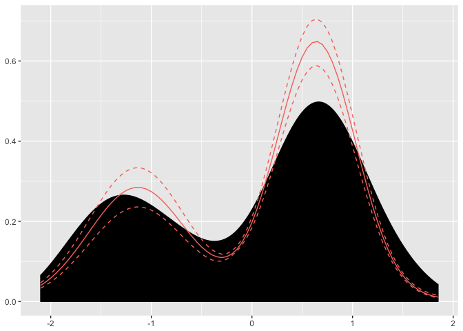
Here we can see the posterior mean of the found distribution and the associated credible intervals. We can look inside the dp object and find the associated cluster parameters.
data.frame(Weights=dp$weights,
                  mu=c(dp$clusterParameters[[1]]),
sigma=c(dp$clusterParameters[[2]]))| Weights | mu | sigma |
|---|---|---|
| 0.330882353 | -1.1438152 | 0.4813677 |
| 0.617647059 | 0.6408545 | 0.3890984 |
| 0.047794118 | 0.3068369 | 0.9846167 |
| 0.003676471 | 0.4765865 | 2.4478375 |
From the weights, we can see that 60% of the data points are associated with a \(\mu = 0.64, \sigma = 0.39\) cluster parameter.
If we want to plot our posterior estimate against our original histogram, we simply have to obtain samples of the posterior distribution.
xGrid <- seq(-3, 3, by=0.01)
postSamples <- data.frame(replicate(100, PosteriorFunction(dp)(xGrid)))

postFrame <- data.frame(x=xGrid, y=rowMeans(postSamples))ggplot() + geom_histogram(data=data.frame(x=faithfulTrans), aes(x=x, y=..density..), binwidth = 0.25) + geom_line(data=postFrame, aes(x=x,y=y), colour='red')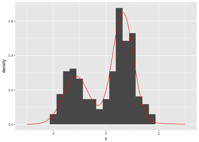
So there we have it. We have successfully modelled the faithful waiting times as a infinite mixture of Gaussian distributions using a Dirichlet process without needing to know any of the underlying algorithms inferring the parameters. All thanks to the dirichletprocess package.
This tutorial is a simplified version of the vignette from the dirichletprocess package. If you want more maths, more examples or more details check that out here