A Hierarchical Model for Yellow Cards
In an older blog
post I looked
at how fitting Bayesian GAM’s are a piece of cake using rstanarm. I
needed an excuse to explore hierarchical models, so using this post as a
way of showing you how you can fit and explore such models using
rstanarm.
I’ve chosen to apply a hierarchical model to the number of yellow cards in English football matches. Using only the referee on the game as the predictor I will show how we can use hierarchical pooling to get a better idea of how a referee can affect the number of cards in a game.
We will be making use of a number of popular packages.
require(readr)
require(dplyr)
require(tidyr)
require(ggplot2)
require(rstanarm)
require(lubridate)
require(stringr)
source("../Betting/BettingFunctions.R")
knitr::opts_chunk$set(cache=TRUE)
rawData <- loadBulkData(leaguePattern = "E")
Using the data from https://www.football-data.co.uk/ we select all the English games from the 2015/16 season onwards. Why? The names of the referees are most consistent from this point onwards. Using older seasons would have meant too much data cleaning for this humble post.
rawData %>%
  select(Div, Date, HomeTeam, AwayTeam, Referee, HY, AY, HR, AR) %>%
  drop_na(Referee) %>%
  mutate(Date=dmy(Date)) %>%
  filter(Date >= dmy("01-08-2015")) -> refereeFrame
glimpse(refereeFrame)
## Observations: 6,636
## Variables: 9
## $ Div      <chr> "E0", "E0", "E0", "E0", "E0", "E0", "E0", "E0", "E0",...
## $ Date     <date> 2015-08-08, 2015-08-08, 2015-08-08, 2015-08-08, 2015...
## $ HomeTeam <chr> "Bournemouth", "Chelsea", "Everton", "Leicester", "Ma...
## $ AwayTeam <chr> "Aston Villa", "Swansea", "Watford", "Sunderland", "T...
## $ Referee  <chr> "M Clattenburg", "M Oliver", "M Jones", "L Mason", "J...
## $ HY       <int> 3, 1, 1, 2, 2, 1, 1, 2, 2, 4, 2, 4, 1, 2, 2, 1, 1, 1,...
## $ AY       <int> 4, 3, 2, 4, 3, 0, 3, 4, 4, 1, 2, 2, 2, 1, 2, 2, 3, 1,...
## $ HR       <int> 0, 1, 0, 0, 0, 0, 0, 0, 0, 0, 0, 0, 0, 0, 0, 0, 1, 0,...
## $ AR       <int> 0, 0, 0, 0, 0, 0, 0, 0, 0, 0, 0, 0, 0, 1, 0, 0, 0, 0,...
We are left with 6636 observations. More than enough to get started.
We create two dataframes, one that has the total number of yellow cards in each match and another that calculates the total number of games each referee has officiated in the dataset. This will come in handy later.
refereeFrame %>%
  select(Div, Referee, HY, AY) %>%
  mutate(ID=seq_len(nrow(refereeFrame)), TotalYellow=HY+AY) %>%
  select(-HY, -AY) -> yellowFrame

refereeFrame %>% group_by(Referee) %>% tally() %>% arrange(-n) -> tallyFrame
Graphs
We plot some exploratory graphs to get a feel for the data.
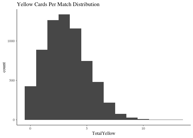
ggplot(yellowFrame, aes(x=TotalYellow)) + geom_histogram(binwidth = 1) + ggtitle("Yellow Cards Per Match Distribution")
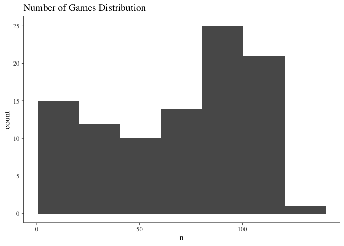
ggplot(tallyFrame, aes(x=n)) + geom_histogram(binwidth = 20, boundary=0.5) + ggtitle("Number of Games Distribution")
The total number of yellow cards per match is has no cause for concern. A Poisson model will suit us just fine for the glm.
The total number of games though is more interesting. There is a large variation in the number of games that each referee has officiated to date. 15 referees have done less that 20, whereas there is also about 25 referees that have officiated 100+ games, the veterans of the game. When we use a hierarchical model we are able to use the information of the veteran referees to help us lear, the parameters of the less experienced refs. This is the key point of hierarchical modelling - the pooling of information.
Modelling
Using rstanarm we fit two models, one where there referee is a free
parameter and one where it is a hierarchical parameter. This is very simple
to forumlate using the R model syntax.
refereeModel <- stan_glm(TotalYellow ~  Referee,
                         data=yellowFrame, family="poisson",
                         chains=2, iter=1500, cores=2)
## Warning: Markov chains did not converge! Do not analyze results!
refereeHierModel <- stan_glmer(TotalYellow ~  (1|Referee),
                               data=yellowFrame, family="poisson",
                               chains=2, iter=1500, cores=2)
The code (1|Referee) indicates that we are imposing a hierarchy of the
referee parameter.
where each referee has a parameter \(\beta_i\) that is drawn from some normal distribution. For referees with little information, we expect their \(\beta _ i \approx 0\). Referees that have a parameter that fall outside the normal range of the prior distribution could indicate that they have a large effect on the number of cards in the game.
After fitting the model without a hierarchy, rstanarm is alerting us
that the chains have not converged, which would be an issue if we
intended to analyse the results of such a model. As we are just using it
as a comparison tool, this lack of convergence is not of major
concern.
We collect the coefficients of the models into data frames. At the minute we will just be using the posterior means from both models.
coefficients(refereeModel)[-1] + coefficients(refereeModel)[1] -> nopool

data.frame(NoPool=nopool,
           Referee=names(coefficients(refereeModel)[-1])) -> nopoolFrame

nopoolFrame %>%
  mutate(Referee = sub("Referee", replacement = "", Referee)) -> nopoolFrame

coefficients(refereeHierModel)$Referee %>% as.data.frame %>% cbind(Referee=rownames(.), .) -> partialpool

left_join(partialpool, nopoolFrame, by="Referee") -> fullFrame
## Warning: Column `Referee` joining factor and character vector, coercing
## into character vector
fullFrame$NoPool[1] <- coefficients(refereeModel)[1]

names(fullFrame) <- c("Referee", "PartialPool", "NoPool")

fullFrame %>% gather(Model, Value, -Referee) -> fullFrameTidy
To understand the effects of pooling we look at the referees who have officiated the most games and those that have officiated the least.
tallyFrame %>% head(5) -> top10
tallyFrame %>% tail(5) -> bottom10
fullFrameTidy %>% filter(Referee %in% top10$Referee) -> topTidy
fullFrameTidy %>% filter(Referee %in% bottom10$Referee) -> bottomTidy
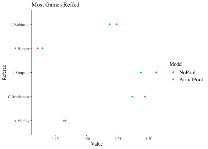
ggplot(topTidy, aes(x=Referee, y=Value, colour=Model)) + geom_point() + coord_flip() + ggtitle("Most Games Reffed")
ggplot(bottomTidy, aes(x=Referee, y=Value, colour=Model)) + geom_point() + coord_flip() + ggtitle("Least Games Reffed")
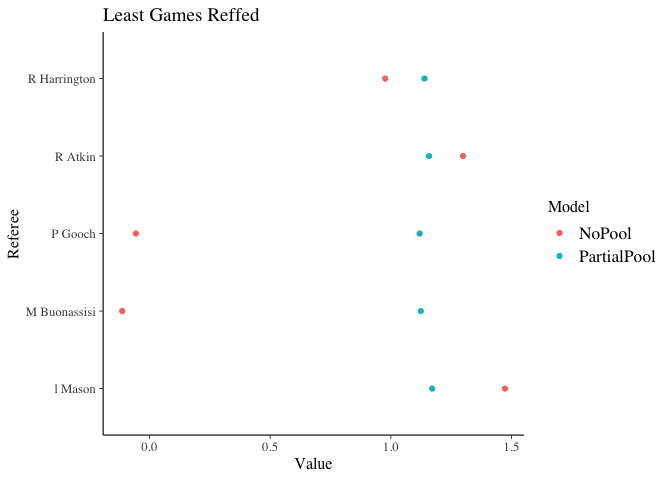
Here we can see that those that have not reffed many games have a major shift in their rate for the partially pooled model as expected. Whereas those that have officiated the most games see little impact in their parameter.
This highlights the power of pooling. Using all the information we are able to better understand the impact of a referee, with less sensitivity on the number of games they have refereed.
Performance Analysis
Are they are any referees that are significantly different from the mean? By this, we want to investigate what referees have a coefficient that falls outside the common distribution.
From the model we know that each referee parameter is distributed as \(\beta _i \sim N(0, \sigma ^2)\) therefore, if a referee’s parameter falls outside a range defined by \(\sigma\) we can conclude that they are having an above average impact on the number of yellow cards in the game. This time we will be using the full posterior samples of the referee parameters.
hierSamples <- as.matrix(refereeHierModel)
sigmaParams <- hierSamples[,ncol(hierSamples)]
refereeParams <- as.data.frame(hierSamples[,-c(1, ncol(hierSamples))])

refereeParams %>%
  gather(Referee, Value) %>%
  mutate(Referee = str_extract(Referee, "[A-z]_(.*)\\w")) -> refereeParamsTidy
We now want to find all the referees that have parameter samples significantly outside the the distribution range. In this case we will borrow from physics and say that if the interquartile range is further than \(5\sigma\) away from 0, then this is evidence that the referee changes the number of yellow cards in a game.
refereeParamsTidy %>%
  group_by(Referee) %>%
  summarise(Mean=mean(Value),
            Abs=abs(Mean),
            LQ=quantile(Value, prob=0.25),
            UQ=quantile(Value, prob=0.75)) -> refAverageParam

refAverageParam %>%
  filter(UQ > 5*mean(sigmaParams) & LQ > 5*mean(sigmaParams)) %>%
  mutate(Referee = gsub("_", " ", Referee)) -> aboveAvg

refAverageParam %>%
  filter(LQ < -5*mean(sigmaParams) & UQ < -5*mean(sigmaParams)) %>%
  mutate(Referee = gsub("_", " ", Referee)) -> belowAvg

bind_rows(aboveAvg, belowAvg) -> refereeOutliers

left_join(refereeOutliers, tallyFrame) %>% arrange(-Abs, -n) %>% knitr::kable(.)
## Joining, by = "Referee"
| Referee | Mean | Abs | LQ | UQ | n |
|---|---|---|---|---|---|
| S Martin | -0.210 | 0.210 | -0.243 | -0.174 | 105 |
| N Miller | -0.202 | 0.202 | -0.244 | -0.156 | 62 |
| K Stroud | 0.198 | 0.198 | 0.163 | 0.232 | 105 |
| E Ilderton | -0.188 | 0.188 | -0.232 | -0.144 | 72 |
| L Probert | -0.177 | 0.177 | -0.218 | -0.137 | 57 |
| P Bankes | 0.176 | 0.176 | 0.146 | 0.210 | 111 |
| M Coy | -0.170 | 0.170 | -0.221 | -0.115 | 37 |
| M Heywood | 0.148 | 0.148 | 0.112 | 0.184 | 85 |
| J Simpson | 0.144 | 0.144 | 0.113 | 0.175 | 114 |
| D Webb | -0.143 | 0.143 | -0.181 | -0.106 | 109 |
| M Jones | 0.142 | 0.142 | 0.101 | 0.179 | 81 |
| T Nield | -0.142 | 0.142 | -0.191 | -0.092 | 33 |
| R Joyce | 0.136 | 0.136 | 0.105 | 0.170 | 109 |
| K Hill | 0.134 | 0.134 | 0.089 | 0.176 | 30 |
| C Breakspear | 0.127 | 0.127 | 0.090 | 0.160 | 113 |
| A Woolmer | -0.124 | 0.124 | -0.165 | -0.082 | 73 |
| D Coote | 0.123 | 0.123 | 0.086 | 0.160 | 97 |
| A Taylor | 0.114 | 0.114 | 0.081 | 0.146 | 98 |
| C Sarginson | -0.112 | 0.112 | -0.147 | -0.077 | 102 |
| J Linington | 0.109 | 0.109 | 0.075 | 0.143 | 91 |
| M Dean | 0.096 | 0.096 | 0.066 | 0.128 | 102 |
| A Davies | 0.094 | 0.094 | 0.060 | 0.130 | 100 |
| T Robinson | 0.093 | 0.093 | 0.059 | 0.124 | 125 |
These are the referee’s that differ from the average significantly. There are a total of 23 which is 23.47% of the data. Based on our model, these are the referees that have an impact on the number of yellow cards in the game. The impact can be both increasing and decreasing the number of cautions shown.
Conclusion
This post has shown how a hierarchical model can be easily fitted using
the rstanarm package. I’ve applied it to the number of yellow cards in
a football match and found that there ar ea number of referees who differ
from the group average. The hierarchical model has been useful in this
case, as there are a wide number of games that different referees have
officiated. By pooling this information, the referees with fewer games
have been pulled towards the group mean and those with more games are
less effected by the pooling. Overall, its been a good exercise to
understand the benefits of a Bayesian approach.