Hidden Markov Models using a Dirichlet Process
Using my dirichletprocess package I have implemented a hidden Markov
model from “Dirichlet Process Hidden Markov Multiple Change-point
Model” [1] . You can build a hidden Markov model using a Dirichlet process
with the components from my dirichletprocess package.
Enjoy these types of posts? Then you should sign up for my newsletter.
set.seed(2019)
require(dirichletprocess)
require(ggplot2)
require(ggExtra)
A Markov Model
Given we have some data \(y_t\) with \(t=1,\ldots,n\) and some unobserved states \(s_t\). We believe that the data is drawn from some distribution that depends on the state
\[y_t \mid s_t \sim p(y_t \mid s_t, \theta _t),\]such that each state has some parameter \(\theta _t\) associated with it. Like a Dirichlet process, these \(\theta _t\)s might be the same.
Typically in a Markovian model, the number of states allowed is fixed. However, in this case, there is a no theoretical limit to the number of states and instead the appropriate number is learnt from the data. This is one of the benefits of using a Dirichlet process - the number of states can be learnt from the data.
Also, a Markov model is usually defined by a transition matrix, where each entry contains the probability of moving from that state. In the Dirichlet case, we parameterise the states by \(\alpha\) and \(\beta\). \(\alpha\) describes the stickiness of a state and \(\beta\) controls the tendency to explore more states.
Hidden Markov Model Inference
In the paper [1] they detail a Gibbs sampler that can be summarised as follows:
- Sample the states \(s_t\)
- Sample the state parameters \(\theta_t\) using the data assigned to that state \(y_t\)
- Sample the hyper parameters i.e. \(\alpha, \beta\).
Steps 2 is simple enough, it is just a case of collecting all the data
associated with the state and sampling from the posterior distribution.
This is all possible using the MixingDistribution objects without any
intervention needed from the user.
Step 3 is also simple. This just requires the posterior which is written in the paper as
\[p(\alpha, \beta) \propto \text{Gamma} (a _{\alpha}, b_{\alpha}) \text{Gamma} (a _{\beta}, b_{\beta}) \prod _{i=1} ^{k+1} \frac{\beta \Gamma (\alpha + \beta)}{\Gamma (\alpha)} \frac{\Gamma (n_{ii} + \alpha)}{\Gamma (n_{ii} + 1 + \alpha - \beta) },\]this can then easily be sampled from using Metropolis Hastings or whatever algorithm you chose.
Its the first step that required the most work in implementation.
Sampling the States
We have left to right transition restriction. Which means that each state can either stay in the current state or move into a new state if it is next to the new state. It can’t form a new state on its own in the middle of another state.
This reduces the amount of computation needed, as we now only need to sample at points where the state changes. Sampling state \(s_t\) is only needed if \(s_{t-1}\) and \(s_{t+1}\) are different. The full derivation of the transition probabilities can be found in the paper, for now, the simplified versions can be written as
\[\begin{aligned} pr(s_t = i-1) & = \frac{n_{ii} + \alpha}{n_{ii} + 1 + \beta + \alpha} p(y_t \mid \theta _{i-1}), \\ pr(s_t = i+1) & = \frac{n_{i+1i+1} + \alpha}{n_{i+1i+1} + 1 + \beta + \alpha} p(y_t \mid \theta _{i+1}), \end{aligned}\]where \(n_{ii}\) counts the number of self transitions for state \(i\) and \(n_{i+1i+1}\) counts the number of self transitions for state \(i+1\).
From these equations we can see that the probability of transition is likelihood of the data with the parameters of the state multiplied by the number of transitions in that state. This shows how the Dirichlet process emerges from the states. Popular states are likely to remain popular.
This took a little bit of effort to write in my package. But it follows the same general process as the normal Dirichlet process inference process. Calculate likelihoods and weight the states by their popularity.
Synthetic Data Example
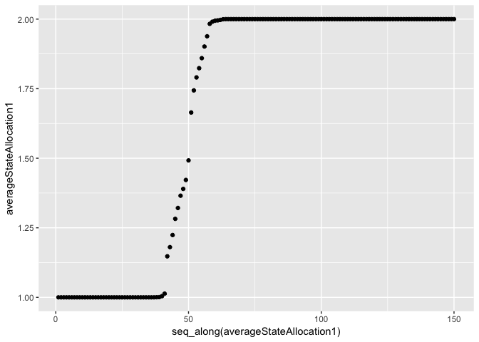
In the paper [1] they use two synthetic examples. In each cases the data is generated from a normal distribution with different means. The first dataset changes once and the second changes twice.
y1 <- c(rnorm(50, 1, sqrt(3)), rnorm(100, 3, sqrt(3)))
y2 <- c(rnorm(50, 1, sqrt(3)), rnorm(50, 3, sqrt(3)), rnorm(50, 5, sqrt(32)))
Rather than write a separate constructor for each type of model, we can
use a generic creator method and just pass in the appropriate
MixingDistribution object. We also give the model starting \(\alpha\)
and \(\beta\) values.
its <- 50000
mdobj <- GaussianMixtureCreate()

dp1 <- DirichletHMMCreate(y1, mdobj, alpha = 1, beta = 1)
dp1 <- Fit(dp1, its, progressBar = F)

dp2 <- DirichletHMMCreate(y2, mdobj, alpha = 1, beta = 1)
dp2 <- Fit(dp2, its, progressBar = F)
To analyse the results we take the samples of the states and calculate the average state assignment value. We remove the first half of the iterations as burnin.
averageStateAllocation1 <- rowMeans(data.frame(dp1$statesChain[-(1:its/2)]))
averageStateAllocation2 <- rowMeans(data.frame(dp2$statesChain[-(1:its/2)]))

qplot(x=seq_along(averageStateAllocation1), y=averageStateAllocation1, geom="point")
qplot(x=seq_along(averageStateAllocation2), y=averageStateAllocation2, geom="point")
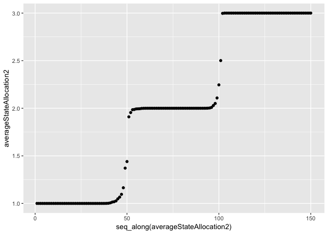
We can see that the correct states have been found. The model is correctly picking up where the data changes distribution.
At the minute, the plotting and printing functions are yet to be
written. But we can hand craft our plots using ggplot and ggExtra.
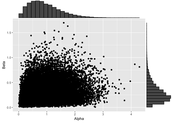
Here we plot the concentration parameters of both of the datasets.
dp1ConcParams <- data.frame(Alpha=dp1$alphaChain[-(1:its/2)], Beta=dp1$betaChain[-(1:its/2)])
dp1Plot <- ggplot(dp1ConcParams, aes(x=Alpha, y=Beta)) + geom_point()
ggMarginal(dp1Plot, type="histogram")
dp2ConcParams <- data.frame(Alpha=dp2$alphaChain[-(1:its/2)], Beta=dp2$betaChain[-(1:its/2)])
dp2Plot <- ggplot(dp2ConcParams, aes(x=Alpha, y=Beta)) + geom_point()
ggMarginal(dp2Plot, type="histogram")
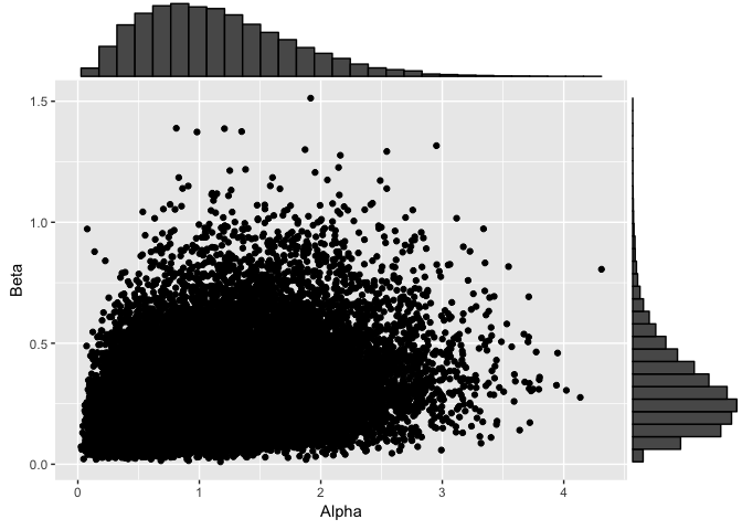
Both have similar values for both of the concentration parameters which is expected, not too much difference between one and two change points.
Conclusion
Using the foundations of the dirichletprocess package I have easily
built and implemented some new functions for fitting a hidden Markov
model. Using the framework from [1] it has been a simple process of
adapting the existing functionality of the package to provide a new
type of model. Give it a try on your data and see if a hidden Markov
model works!
If you want a practical example you can read where I apply this type of model to the stock market and how we can come up with the state of the market. If you prefer a video, I’ve done a quick talk for UseR 2021: https://www.youtube.com/watch?v=6kSPwHcO6L0