Posterior p-values
I am now at the point in my work where I need to check my models and whether they correctly describe the data. To do this, lets introduce posterior p-values for a Bayesian model.
Say we have data \(y\) that we fit using a model \(F\) with parameters \(\theta\). As we would have used MCMC to fit the model we have chain of parameter values \(\{\theta ^{(0)} ... \theta ^{(n)}\}\).
For each parameter value we can obtain simulated data \(\hat{y} _i = F( \theta ^{(i)})\) such that we now have \(n\) simulated data sets.
We now chose a test statistic, \(T\) and calculate it for each simulated data set. We can now how \(T_{\text{real}}\) compares to the \(T_{\text{sim}}\). If \(T_{\text{real}}\) is drastically different from the simulated \(T\)’s then there is a problem with our model, it is not correctly picking up something intrinsic to the real data.
Like all good introductions, lets add some real data to try and explain the concepts better.
Our real data will be simulated from the Generalised Pareto distribution (gpd) and we will fit both an exponential model and a gpd model.
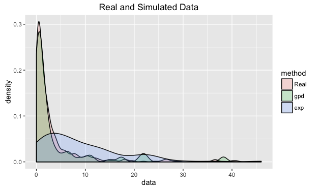
So now we have three data sets, \(y_{\text{real}}, \hat{y}_{\text{gpd}}, \hat{y}_{\text{exp}}\).

We can see straight away that the gpd model has nicely replicated the general shape of the real data, where as the exponential model has produced a poor fit.
Now we chose a test statistic, \(T\). For simplicity we shall use the maximum value of the data set, \(T(x) = \max x_i\).
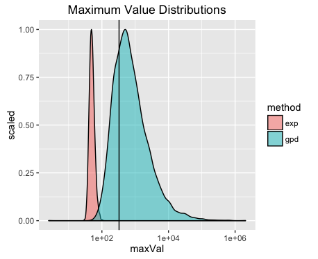
So we now calculate the maximum value for all our simulated datatsets of both models and see how the maximum of the real data compares.

The solid black line in the maximum value of the real data set and just by inspection we can reasonably assume that the data is best modelled using a gpd model. Even more so as the x-axis is on a log scale!.
So this test statistic appears to be suitable of discerning if the data comes from a gpd.
Now by doing some maths you can calculate the usual power and size of the test statistic, but I’ll save that for a another blog post. This also shows how this method can seem analogous to frequentist p-values.
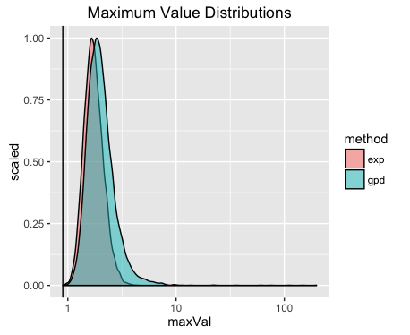
Now, lets try using the same method but this time the real data is going to come from an exponential distribution.

Here our test statistic has failed. This is no obvious difference between the two distributions of the maximum value for the models. Therefore we can not conclude anything. A better test statistic is required!
So overall, we have shown how to utilise basic test statistics and simulated datasets to analyse the suitability of a model.
References:
http://www.stat.columbia.edu/~gelman/research/published/A6n41.pdf
The Big Red Book of Bayesian Data Analytics (Bayesian Data Analytics by Gelman et al.)