Bayes Comp 2018
This time last month I was in Barcelona for BayesComp 2018 at Universitat Pompeu Fabra (UPF). A conference dedicated to Bayesian statistics and the challenges it poses; from large data sets, different types of priors and upcoming software packages. I learnt quite a bit and in this post I’ll outline some of those new things.
Through my work, I’ve only ever used random walk Metropolis Hastings algorithms. Therefore the convergence of my MCMC chains can be problematic as we are jumping around with little information. Step forward the Metropolis adjusted Lagenvin algorithm (MALA). This uses the gradient of the likelihood function to make sure your sample steps are moving in the correct direction. Therefore the next proposed step in the sample can be written as
\[x_{k+1} = x_{k} + \tau \nabla \log \pi (x_k) + \sqrt{2 \tau} \xi,\]where the likelihood is \(\pi (x)\), \(\tau\) is the size of the jump and \(\xi\) is some Gaussian noise. This extra piece of information can help make sure your MCMC chains move towards areas of high probability quicker and thus sample the unknown distribution better. This comes at a cost though. You need to be able to easily calculate the gradient of your likelihood function. For most distributions, this is easily specified, but as models become more complicated, so do the gradients. Like most things, its a case of balancing the complexity with the performance increase. For my R package, dirichletprocess, it is something we can look at implementing for the non-conjugate models, but we need to make sure that it remains customisable.
My favourite talk from the conference was “Coresets for automated scalable Bayesian inference” by Tamara Broderick. In essence, we can speed up our MCMC computations by using only the most ‘important’ data points from the sample. How do we chose what the important data-points are? By looking at their influence on the total likelihood. We then give each data point a weight (that could be 0) and calculate the ‘coreset’ likelihood.
\[L_i = \ln p ( x_i \mid \theta ), \\ L = \sum _{i=1} ^N L_i, \\ L_{\text{coreset}} = \sum _{i=1} ^N w_i L_i,\]we can then perform the MCMC on this coreset likelihood which will run quicker that the performing a full sample on all the data. In practice, choosing the weights \(w_i\) is non-trivial and the excellent talk outlined the methods which can be employed to make sure the coreset likelihood is the best possible approximation. Again, applying this to my dirichletprocess package, using all the datapoints in each cluster doesn’t scale, instead, being able to for a coreset for each cluster could lead to significant performance increases.
There was a session on Bayesian statistics in physics, which was a nice throwback to my undergrad days. Modelling the composition of exoplanets using Bayesian hierarchical modelling was a nice applied talk and interesting to see how both the fundamentals of planet formation and statistics can be combined. Using first principles can help specify priors and highlight the uncertainty of observations.
The current offerings of Bayesian software was also demonstrated. NIMBLE a package for specifying a vast array of models and inferring them. The lead of NIMBLE actually enquired about implementing my Dirichlet process package in there framework, which was exciting.
Overall, I expanded my knowledge of Bayesian computation and have been inspired to try some new approaches in my work. I can definitely seeing coresets being useful in the future, and its always good to add another sampling algorithm such as MALA to my arsenal. Bring on the next conference, which will be ISBA in Edinburgh.
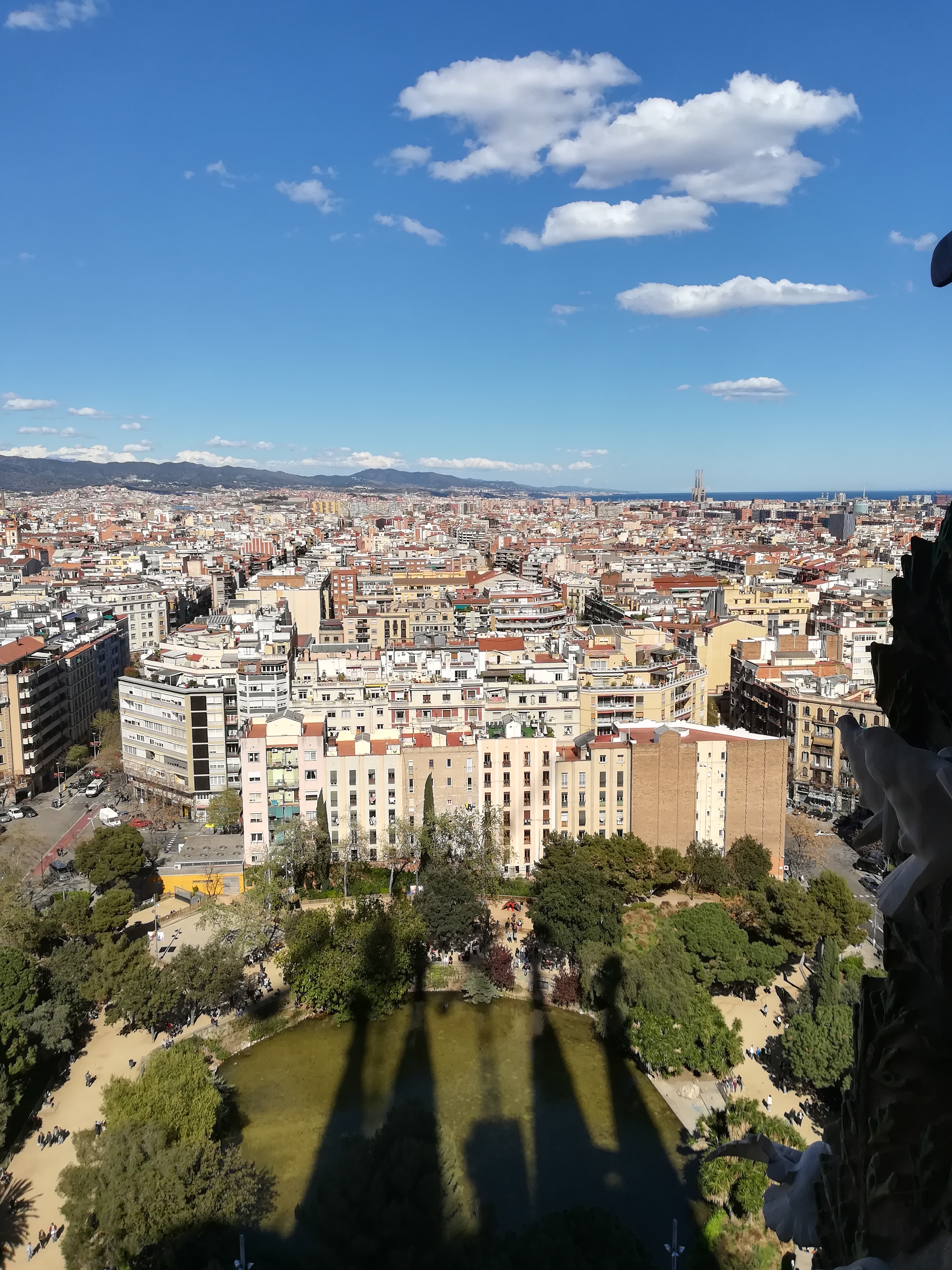
Bonus shot of the Sagrada Famillia view from the Nativiety Tower. Pretty cool that you can make out the distinctive shape of the Cathedral in the shadow. Plus a crane.