How Tough is that Football Match?
How do we quantify the difficulty of a soccer match and can we construct a single number that will explain how easy or hard the match is for a team to win? I think we can approach this by looking at the match odds and coming up with a way to measure the imbalance. If one team is a dead certain favourite to win, then that match should be easy for them and difficult for their opponent. If the odds are similar for either team, then the match is balanced and their is no apparent difficulty for either side.
Enjoy these types of posts? Then sign up for my newsletter.
Kullback–Leibler Divergence
The Kullback-Leibler divergence is a fancy method of comparing how two probability distributions are different. It has a vast array of applications and can be used in lots of different contexts, from time series analysis to machine learning model fitting. In our case we are using it to compare the match outcome probability distribution to a reference distribution.
For each match there is a probability distribution, \(p_\text{win}, p_\text{draw}, p_\text{lose}\) which we can derive from the match odds. What we want to know is how far away is this probability distribution from a uniform distribution, where each outcome has an equal chance. Kullback-Leibler Divergence (KL Divergence) does this calculation and summarises how the probability distribution \(p\) is different from the probability distribution \(q\) and is calculated as
\[\text{K} = \sum _i p_i \log \frac{p_i}{q_i},\]where \(p_i\) and \(q_i\) are the probabilities in question for each outcome. Our match probability distribution (\(p\)) will be calculated from the odds of the match, the reference distribution (\(q\)) will be 1/3 for each outcome. This will give us one number that describes how different the match outcomes are from the uniform distribution.
Right enough maths. Onto the data.
Once again we turn to www.football-data.co.uk to download the results from many leagues across the years. We then convert the Pinnacle closing odds into probabilities \(\left( p ^{\text{raw}} = \frac{1}{\text{Decimal Odds}} \right)\) using the standard normalisation procedure
\[p_i = \frac{p_i ^\text{raw}}{\sum _i p ^ \text{raw} _i}.\]Once that is done, we can calculate the KL divergence for each match with our reference uniform distribution across the three outcomes.
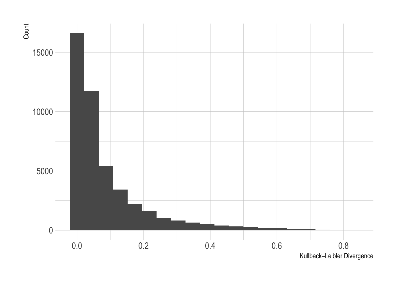
Here is the distribution of the KL divergence values across the dataset. Most values are concentrated around 0 with a long decay out to the larger values.
- Competitive matches have a KL divergence \(\rightarrow 0\) as each of the outcomes has an equal chance to happen.
- One sided matches have a KL divergence \(\rightarrow 1\) as there is a clear favourite that is likely to win. The match outcome odds are unbalanced.
To hammer the point home: a KL divergence of 0 indicates that the match outcome was close to even, i.e. 1/3 chance home team win, 1/3 chance away team win, 1/3 chance draw. A KL divergence approaching 1 indicates that one team had a much higher chance than the other of winning the match.
To add some context I’ve pulled out the largest and smallest KL values to see what matches they represented.
| Date | HomeTeam | AwayTeam | PSCH | PSCD | PSCA | KL |
|---|---|---|---|---|---|---|
| 2014-03-02 | Barcelona | Almeria | 1.05 | 22.50 | 51.00 | 0.82 |
| 2018-01-28 | Leganes | Espanol | 2.91 | 2.93 | 2.94 | 0.00 |
Barcelona vs Almeria is the easiest match in the database with the largest KL value of 0.82 as Barcelona were the clear favourites at 1.05. On the other side of the coin Leganes vs Espanol in 2018 was the most evenly matched where each outcome was equal and a KL divergence of 0 (rounded to two decimal places). In this match, each of the outcomes had very similar odds. Also, funny to note how both matches involved Spanish teams.
From a KL Divergence to a Match Difficulty
The KL divergence value shows how unbalanced a match was, but to convert it into a difficulty metric we need to understand who the better team is in the match, our more typically put, the favourite. Again, we can simply use the odds and multiply the KL divergence by 1 or -1 depending on whether the team is the favourite or the underdog.
So the full calculation steps are as follows:
- Calculate the probability of each match outcome using the match odds.
- Calculate the KL divergence, \(K\), of this distribution compared to a uniform distribution.
- For the match favourite (likely winner) the match difficulty is \(K\).
- For the other team the match difficulty is -\(K\).
Fixture Difficulty Per Team
Each team now has a difficulty rating for each of the matches it has played in the database. We can go through each team, calculate a rolling average to smooth the data out and see how each team’s difficulty rating has changed over time.
Dominant teams are going to have a difficulty rating greater than zero, reflecting how they are usually favourites going into each match, whereas weaker teams, will have a negative average difficulty. If a team can sustain a high difficulty measure, then this indicates they are performing well.
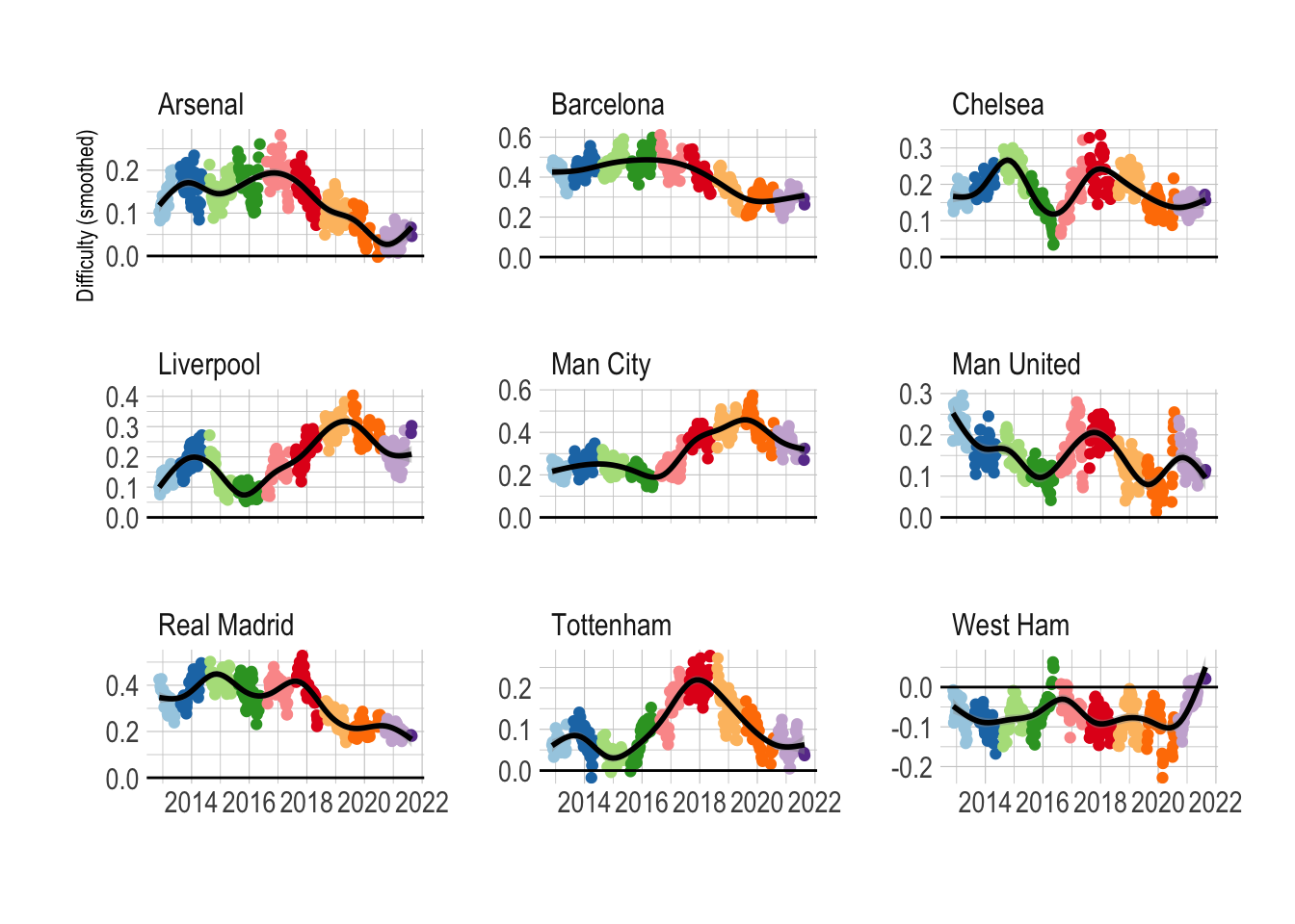
Each colour here represents a different season and I’ve added on a general trend line in black.
Difficulty gives a good indication of a teams ‘dominance’ and condenses everything down into one number that seems to pass the eye test in terms of a teams fortunes. Liverpool have fallen off since their Champions League/title winning seasons. West Ham are going through one of their best periods since (these) records have began. Real Madrid and Barcelona have both come down slightly since their periods of dominance.
League Difficulty
We can also assess the overall league difficulty by calculating the average over a season per league, making sure we only count each match once.
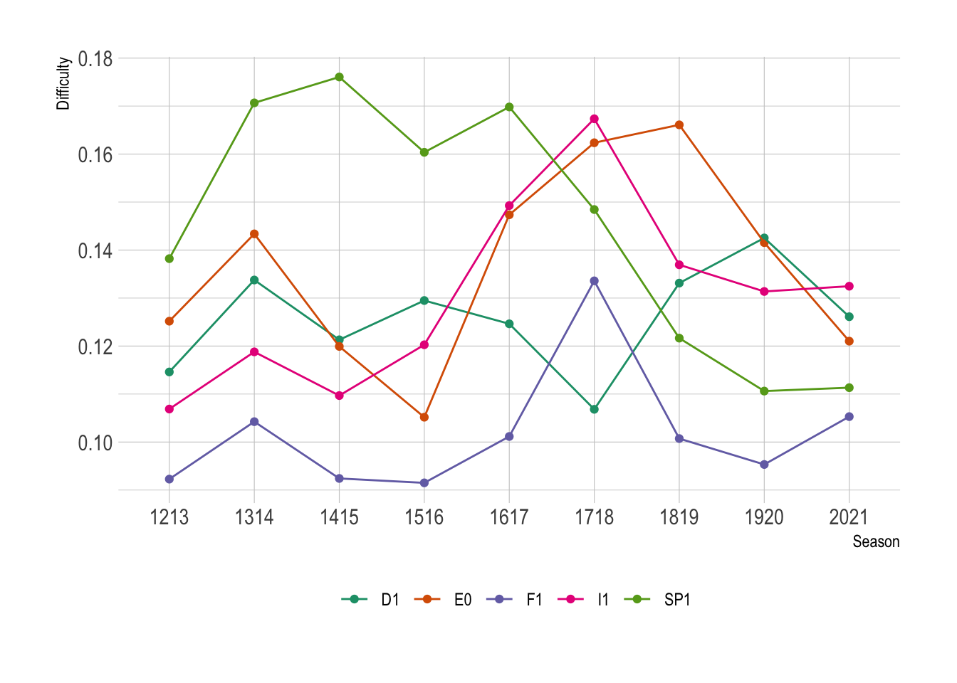
Here we can see Serie A (I1) has the most average difficulty game, whereas Ligue 1 (F1) is the least, which is surprising considering the dominance of PSG. The Premier League (E0) is nicely in the middle. More interesting La Liga (SP1) had been the most difficulty up until 16/17 when is has since balanced out more, perhaps highlighting how the main dominance of Real Madrid and Barcelona has fallen off recently compared the start of the decade.
So we’ve shown that there have been some interesting trends in difficulty across both teams and seasons, but the bigger question is, does is have any predictive power?
Using Match Difficulty to Predict Things
To start with, I’ll predict the outcome of the match using the
difficulty and the odds of the match. We’ve compressed the odds into
one number with the difficulty and now want to map this number
back to a probability of winning. I’ll use the nnet package to build
a multinomial neural net, which is just a single-hidden-layer network,
so nothing too fancy.
I fit three models, one with just the odds, one with the difficulty only and one with both odds and the difficulty. Each of the three models also has a variable for the division that the match was played in with all two way interactions. The result is a factor (-1 for a loss, 0 for a draw and 1 for a win).
require(nnet)

oddsOnly <- multinom(Result ~ (Div + WinProb + DrawProb + LoseProb) ^ 2,
                                      data=trainData)

oddsAndDifficulty <- multinom(Result ~ (Div + Difficulty + WinProb + DrawProb + LoseProb) ^ 2,
                        data=trainData)

difficultyOnly <- multinom(Result ~ (Div + Difficulty ) ^2 ,
                        data=trainData)
The models are trained on all matches before 2020 and tested on all models after 2020.
| Accuracy | Kappa | Model |
|---|---|---|
| 0.496 | 0.211 | Odds and Difficulty |
| 0.496 | 0.210 | Odds Only |
| 0.496 | 0.208 | Difficulty Only |
So not much difference between the models in terms of accuracy or the Cohen’s \(\kappa\) value so I think we can conclude the difficulty of a match doesn’t really add anything. The match difficulty is a second order effect compared to the match outcome probabilities, so unlikely to really improve model performance, its adding minimal amount of information.
Goals and Difficulty
So not much luck in helping predict the outcome of the match, but what about the number of goals in a match?
We are going to model both the goals scored by a team using a Poisson regression model. I’ll just be using the difficulty of the match to predict the number of goals scored, but will use a GAM and a GLM to see if there is a nonlinear dependence. I’ve thrown a null model in there as well, just to make sure the difficulty measure is adding some predictive power.
require(mgcv)
goalsScored_glm <- glm(GoalsScored ~ Difficulty,
family = "poisson", data=trainData)

goalsScored_gam <- gam(GoalsScored ~ s(Difficulty),
familty = "poisson", data=trainData)

goalsScored_null <- nullModel(y=trainData$GoalsScored)
Again, trained on all matches before 2020 and evaluated on all matches after 2020.
| RMSE | Rsquared | MAE | Model |
|---|---|---|---|
| 1.122 | 0.112 | 0.887 | GAM |
| 1.129 | 0.101 | 0.901 | GLM |
| 1.191 | NA | 0.961 | Null |
I evaluate all three models on the held out test set and find that the GAM is the best fitting model across all three metrics. Reduction in the error measures and an increase in the \(R^2\) value. Both models also improve on the null model, so it looks like we are actually onto something with this measure.
Lets plot some graphs and see what the relationship between goals scored and difficulty and how the GLM and GAM differ.
To summarise the data, we round the difficulty to two decimal places and calculate the average goals scored for that difficulty measure.
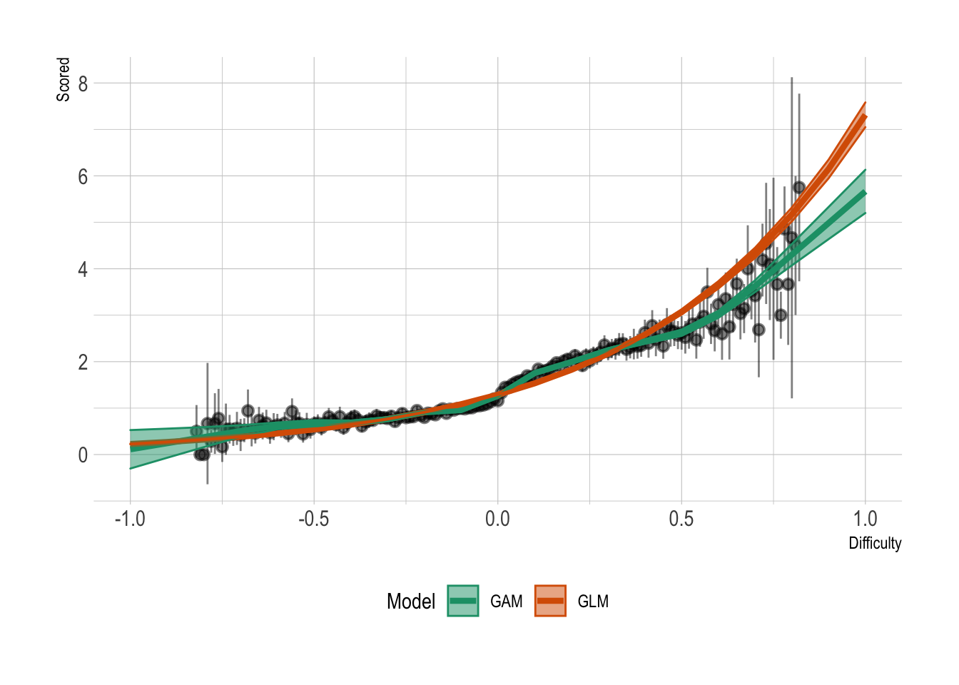
Both models capture the underlying behaviour, but there are extra nonlinear effects that the GAM is able to learn, which gives is the edge over the GLM. For small difficulty values we can see the GLM underestimates. Overall, gives us a good indication that difficulty leads to a change in the number of goals scored and thus through symmetry goals conceded.
Shots and Shots on Target
How does difficulty effect other features of a match? We can repeat the above modeling approach but switching out the dependent variable from goals to shots and shots on target. We stick with a Poisson based model, which is a bit of a large assumption to make as shots and shots on target don’t really follow a Poisson distribution, but for now it will do.
| RMSE | Rsquared | MAE | Model |
|---|---|---|---|
| 10.518 | 0.110 | 10.324 | Shots |
| 3.346 | 0.111 | 3.124 | TargetShots |
| 1.122 | 0.112 | 0.887 | Goals |
All three outputs have a similar \(R^2\) which is what we would expect really as goals, shots and shots on target are all correlated with each other, so difficulty is going to be good at describing them all. We can’t compare the error metrics (MAE, RMSE) across the models, as they are all distributed differently, there is more shots compared to shots on target and also the variation is also larger.
When we plot the nonlinear effect of the difficulty in a match we can see that the shapes are very similar across the three metrics, with goals having a larger variation.
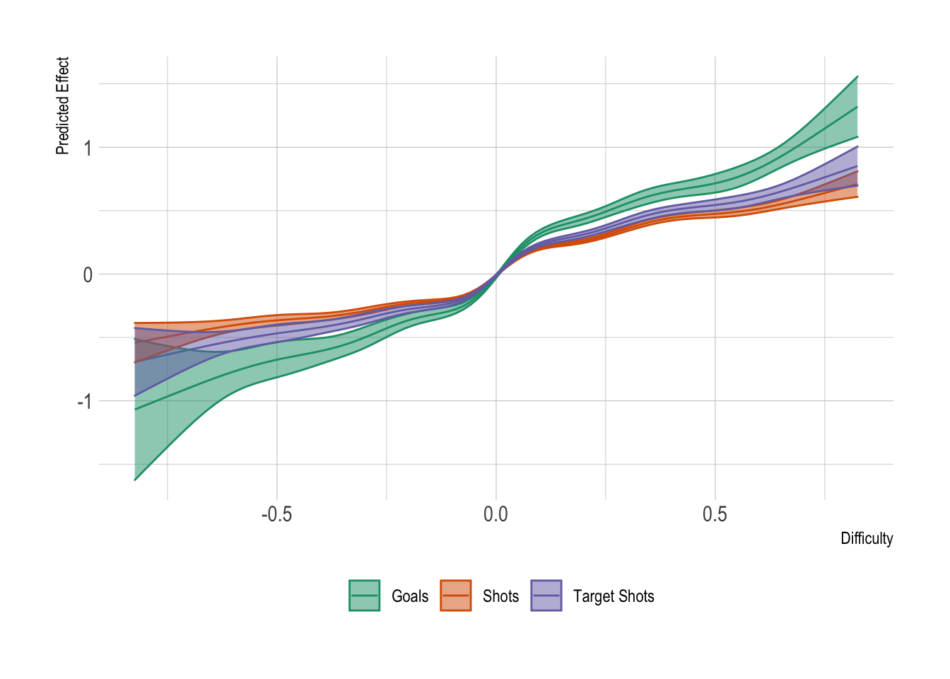
Again, looking at the relationship we can see that goals has the most variation with respect to difficulty. Shots and shots on target are very similar. Similar shapes though, so we can assume that easier matches (difficulty > 0) allow you to generate more shots and shots on target which eventually lead to goals.
Conclusion
Hopefully I’ve convinced you that measuring the KL divergence between the odds gives a good approximation to the difficulty of that fixture. Teams that have easier fixtures tend to score more goals and have more shots, both normal and those on target. This lines up with what we would think would happen in an easier match so I think we can conclude all is well.
In my next post I’ll use this difficulty measure in the Fantasy Premier League setting to see if players score more points in easier or hard matches.
Environment and Footnotes
A bit like shownotes, I’ll describe here how I’ve plotted the graphs.
Unsurprisingly, they’ve all been built in ggplot2 with the ipsum
theme from the hrbrthemes package. In terms of colours, it was trial
and error on the https://colorbrewer2.org website and after choosing
a palette using scale_colour_brewer function.
The models were fitted using nnet (for the outcome model) and mgcv
for the all the GAMs. Nothing fancy.
You can download a notebook that contains all the code here:
You’ll have to download the football data yourself, but then the above can be run.
knitr::opts_chunk$set(warning = FALSE,
                      fig.retina=2)
require(readr)
require(dplyr)
require(tidyr)
require(ggplot2)
require(TTR)
require(knitr)
require(lubridate)
require(caret)
require(mgcv)
require(hrbrthemes)
theme_set(theme_ipsum())
klDiverance <- function(x){
  sum(x * log(3*x))
}