Golf and Online Linear Regression
Golf became the only thing you could do in the COVID times and given my interest in sports modeling I made sure to start recording my scores and different stats about each of my rounds. This post outlines a specific model used in golf called Strokes Gained and relates the number of strokes required at a given distance to get the golf ball in the hole. It is a simple model but can describe someones golfing, or lack of in my case, ability.
Enjoy these types of posts? Then sign up for my newsletter.
Strokes Gained
My inspiration for this type of analysis comes from Matt Broadie’s Strokes Gained metric, available in the Golf Metrics app. For every position around the course, there is an expected number of shots required to finish the hole. So think of an easy par 3 hole, on average, you are expected to take three shots to get the ball in the hole, starting with your tee shot. Now let’s say your first shot is excellent and you land it very close to the hole. On average it takes 1 shot for people to make a putt from that distance, it is that close. Therefore, by doing an excellent tee shot you have ‘gained’ an extra shot.
After taking 1 shot, your tee shot, you have moved from a position of 3 expected strokes to a new position of 1 expected stroke. Therefore your strokes gained is 1.
\[\mathbb{E} [s_1] - \mathbb{E} [ s_2 ] - 1 \\ 3 - 1 - 1 = +1\]The PGA tour has a repository of expected shots from different positions on all the professional courses. I need to come up with a model for my rounds that estimates how many shots it would take for each hole for each of the courses I play. This will form my amateur Strokes Gained estimate.
These are the packages I am using.
require(readr)
require(dplyr)
require(ggplot2)
require(hrbrthemes)
theme_set(theme_ipsum())
extrafont::loadfonts()
require(wesanderson)
source("Golf/load_data.R")
Firstly, I save all my scores in Google Sheets and have a wrapper function to load them into R.
allData <- loadData(cache = F, save=F) %>% filter(Course != "DuntonPar3")
courseData <- loadCourses(cache = F, save=F)
Golf, for those not aware, is about getting a ball in a hole in as few strokes as possible. A golf round is played over 18 holes, each of different distances and difficulty. The holes will be ‘Par X’ which means you are expected to take X shots:
For example, in the last three years:
allData %>%
  filter(Player == "Dean") %>%
  group_by(Par) %>%
  summarise(AvgShots = mean(Strokes), AvgDistance = mean(Yards))
| Par | AvgShots | AvgDistance |
|---|---|---|
| 3 | 4.53 | 157. |
| 4 | 5.97 | 343. |
| 5 | 7.10 | 476. |
I’m between 1.5 and 2 shots over the expected number of shots. We can also see how the average distance of these holes changes, about 100 yards for an increase in expected shots.
When we plot the number of shots vs the yardage of the hole we get a cool picture
ggplot(allData %>% filter(Player == "Dean"),
       aes(x=Yards, y=Strokes)) +
  geom_point(aes(color=as.factor(Par))) +
  geom_smooth(method = "lm") +
  geom_smooth(method = "gam", color="pink") +
  theme(legend.position = "bottom") +
  labs(color = "Par") +
  ggtitle("Strokes vs Yards") +
  scale_color_manual(values = wes_palette("Moonrise2"))

This is a compelling plot - there is a clear and unsurprising relationship between the hole distance and the number of strokes it takes to get it in the hole. Both the linear model (blue) and GAM (red) indicate a simple relationship.
lm(Strokes ~ YardsNorm, data = allData %>%
     filter(Player == "Dean") %>%
     mutate(YardsNorm = Yards/100))
## Coefficients:
## (Intercept)    YardsNorm
##      3.2430       0.8026
This model has an \(R^2\) of 35% and the parameters explain:
-
At 0 yards I’m expected to take 3.24 shots to get it into the hole. So this is a rough approximation of my short game/putting ability.
-
Each additional 100 yards means I take 0.8 shots for this round. Or if we take the reciprocal 125 yards is my average distance per shot.
So for a 400 yards hole, I’m expected to take 6.453 shots. This is a long par 4 and about a double bogey.
Being able to predict the number of shots per hole gives us a good way of looking at my ability per hole and also per round, by summing the 18 individual predictions for a course.
How to Model Over Time?
How do these parameters evolve? I want to be able to understand how my golfing ability had changed over the months and see if I am getting better or worse.
To start with, let’s just pull my data out and label each round using
the cur_group_id function.
allData %>%
  filter(Player == "Dean",
         Course != "DuntonPar3") %>%
  mutate(YardsNorm = Yards/100) %>%
  group_by(Date) %>%
  mutate(ID=cur_group_id()) %>%
  ungroup -> modelData
We can fit a model to each round my using Map and
filtering for each ID.
res <- bind_rows(Map(function (x)
data.frame(t(coef(lm(Strokes~YardsNorm,
                                data=modelData %>% filter(ID == x)))),
                     ID = x),
                     unique(modelData$ID)))
names(res)[1] <- "Intercept"
res$Model <- "SingleRound"
Or we can fit one model to all the rounds.
bigRes <- lm(Strokes ~ YardsNorm, data=modelData)
Or we can incrementally include each round in the models, by including all the data up to a given ID.
res2 <- bind_rows(Map(function (x) data.frame(t(coef(lm(Strokes~YardsNorm, data=modelData %>% filter(ID <= x)))), ID = x),
                     unique(modelData$ID)))
names(res2)[1] <- "Intercept"
res2$Model <- "IncRound"
We create a big data frame with both models.
allRes <- bind_rows(res, res2)
Both models are plotted over the years with a horizontal line that shows the parameter of the big model.
ggplot(allRes, aes(x=ID, y=Intercept, color=Model)) +
  geom_point() +
  geom_line() +
  xlab("Round") +
  ggtitle("Data Lookback") +
  theme(legend.position = "bottom") +
  geom_hline(yintercept = coef(bigRes)[1], aes(color="BigModel")) +
  scale_color_manual(values = wes_palette("Moonrise2"))

The single-round model pings about rather erratically, much like me on the golf course. Whereas incrementally fitting the model on each successive round shows a clearer evolution of the parameters. Both models are centered around the one-shot model (fitting all the data at once), so my golfing ability hasn’t changed too much over the last three years. Bit depressing.
A problem with the incremental model is that the rounds in 2020 have as much weight on the parameters as the rounds in 2022, which doesn’t make that much sense. We need a way of discounting the older rounds.
Online Linear Regression
Online learning is a way of training a model with each new observation rather than relying on a full dataset. This means it can be quicker, as you don’t need the full dataset or its just makes sense practically if your data arrives sequentially. In my case, we want to update the parameters with each new round of golf played. With each round, we update the parameters whilst at the same time discounting the older observations.
We have the number of yards and a constant in our \(X\) matrix, plus the number of shots as a matrix \(Y\), the outcome.
For each round \(t\) we update the using the following
\[M_t = \alpha M_{t-1} + (1-\alpha) X_t ^T X_t,\] \[V_t = \alpha V_{t-1} + (1- \alpha) X_t^T Y_t,\]and our estimated parameters are obtained by:
\[\beta _t = M_t ^{-1} V_t.\]We have to choose an \(\alpha\) value which will control how much influence the older rounds have on the current parameters. This big (and unoptimised) function does the above and also calculates the RMSE so we can optimise later.
recur_reg <- function(modelData, a){

  X <- modelData %>% filter(ID == 1) %>% select(YardsNorm) %>% mutate(Intercept = 1) %>% as.matrix
  Y <- modelData %>% filter(ID == 1) %>% select(Strokes) %>% as.matrix

  dt <- modelData %>% filter(ID == 1) %>% head(1) %>% pull(Date)
  nm <- modelData %>% filter(ID==1) %>% head(1) %>% pull(Player)

  M <- t(X) %*% X
  V <- t(X) %*% Y
  B <- solve(M) %*% V

  s <- (t(Y - X%*%B) %*% (Y - X%*%B)) / (nrow(X) - 2)
  sigma <- as.numeric(s) * solve(t(X)%*%X)
  resM <- list()
  resV <- list()
  resB <- list()
  resRMSE <- numeric(max(modelData$ID))
  resSigma <- list()
  resRMSETrain <- numeric(max(modelData$ID))

  resM[[1]] <- M
  resV[[1]] <- V
  resB[[1]] <- as.data.frame(t(B), row.names = "") %>%
    mutate(Date =dt, Alpha = a, Player = nm, SlopeSD = sigma[1,1], InterceptSD = sigma[2,2], Corr = sigma[1,2])


  resRMSETrain[1] <- as.numeric(s)
  resSigma[[1]] <- sigma


  res350 <- list()
  res350[[1]] <- data.frame(Exp350 = B %*% c(3.5, 1), Date =dt, Alpha =a, Player = nm)

  for(i in 2:max(modelData$ID)){
    X <- modelData %>% filter(ID == i) %>% select(YardsNorm) %>% mutate(Intercept = 1) %>%  as.matrix
    Y <- modelData %>% filter(ID == i) %>% select(Strokes) %>% as.matrix
    dt <- modelData %>% filter(ID == i) %>% head(1) %>% pull(Date)
    M <- a*resM[[i-1]] + (1-a)* t(X) %*% X
    V <- a*resV[[i-1]] + (1-a)* t(X) %*% Y
    B <- solve(M) %*% V

    s <- (t(Y - X%*%B) %*% (Y - X%*%B)) / (nrow(X) - 2)
    sigma <- as.numeric(s) * solve(t(X)%*%X)
    resRMSETrain[i] <- as.numeric(s)
    resSigma[[i]] <- sigma

    if(i != max(modelData$ID)){
      XPred <- modelData %>% filter(ID == i + 1) %>% select(YardsNorm) %>% mutate(Intercept = 1) %>% as.matrix
      YPredTrue <- modelData %>% filter(ID == i + 1) %>% select(Strokes) %>% as.matrix
      YPred <- XPred %*% B
      resRMSE[i] <- sqrt(sum((YPred - YPredTrue)^2))
    }

    resM[[i]] <- M
    resV[[i]] <- V
    resB[[i]] <- as.data.frame(t(B)) %>% mutate(Date =dt, Alpha = a, Player = nm, SlopeSD = sigma[1,1], InterceptSD = sigma[2,2], Corr = sigma[1,2])
    res350[[i]] <- data.frame(Exp350 = t(B) %*% c(3.5, 1), Date = dt, Alpha = a, Player = nm)
  }

  resB <- bind_rows(resB)
  res350 <- bind_rows(res350)

  return(list(params=resB, rmse=resRMSE, res350=res350, rmseTrain = resRMSETrain, sigma=resSigma))
}
What should \(\alpha\) be? We can experiment by looking at different values and judging the output.
res10 <- recur_reg(modelData, 0.1)
res50 <- recur_reg(modelData, 0.5)
res90 <- recur_reg(modelData, 0.9)
We can also optimise the function to find an optimal value. In this case, we minimise the rmse of the next round.
optAlpha <- optimize(function(x) mean(recur_reg(modelData, x)$rmse),
                                   interval = c(0,1))
resOpt <- recur_reg(modelData, optAlpha$minimum)
Joining all the results together.
paramsRes <- bind_rows(res10$params,
                       res50$params,
                       res90$params,
                       resOpt$params)
res350 <- bind_rows(res10$res350,
                    res50$res350,
                    res90$res350,
                    resOpt$res350)
And plotting all the results together again.
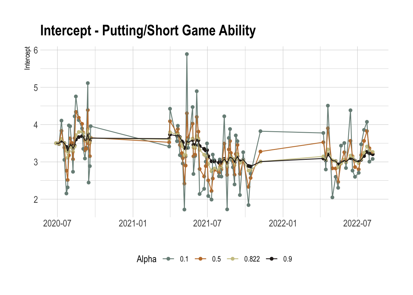
ggplot(paramsRes %>%
         mutate(Alpha = round(Alpha, 3)), aes(x=Date, y=Intercept)) + geom_point(aes(color = as.factor(Alpha))) +
  geom_line(aes(color = as.factor(Alpha))) +
  theme(legend.position = "bottom") +
  xlab("") +
  labs(color = "Alpha") +
  ggtitle("Intercept - Putting/Short Game Ability") +
  scale_color_manual(values = wes_palette("Moonrise2"))
ggplot(paramsRes %>% mutate(Alpha = round(Alpha, 3)), aes(x=Date, y=YardsNorm)) + geom_point(aes(color = as.factor(Alpha))) +
  geom_line(aes(color = as.factor(Alpha))) +
  theme(legend.position = "bottom") +
  xlab("") +
  ylab("Slope") +
  labs(color = "Alpha") +
  ggtitle("Slope - How Many Strokes to get 100 yards") +
  scale_color_manual(values = wes_palette("Moonrise2"))
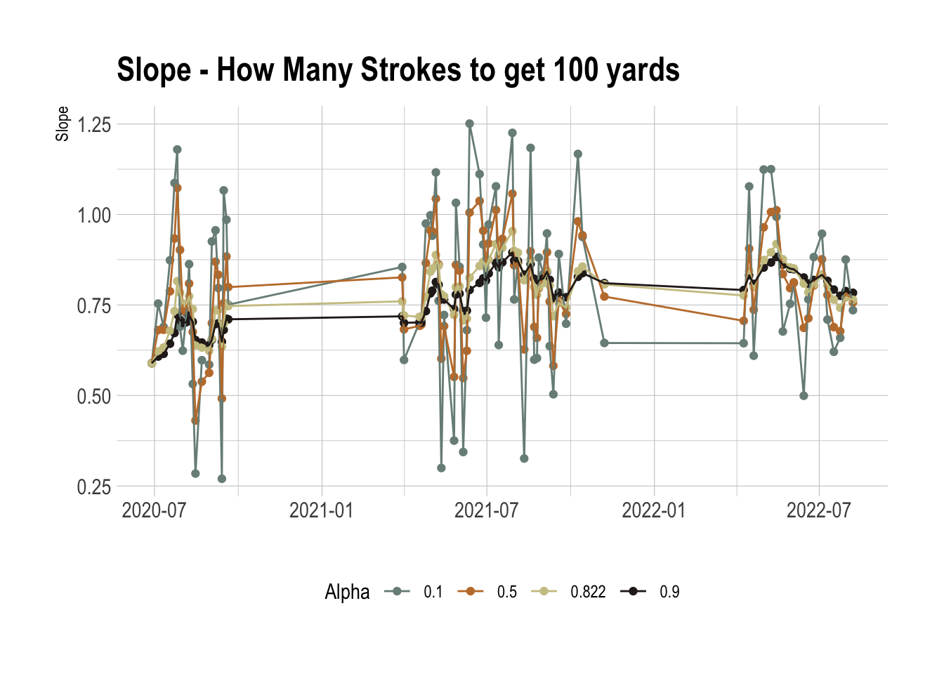
The higher α values allow the parameters to evolve slower and the optimal value is around 0.8. This is interesting as it suggests a relative number of observations around 10 rounds, which is the same as the official World Handicap Rating system, it takes your last 10 rounds into account.
ggplot(res350 %>%
         mutate(Alpha = round(Alpha, 3)) %>%
         filter(Alpha > 0.5), aes(x=Date, y=Exp350)) +
  geom_point(aes(color = as.factor(Alpha))) +
  geom_line(aes(color = as.factor(Alpha))) +
  xlab("") + ylab("Expected Shots") +
  ggtitle("Expected Shots for a 350y Hole") +
  theme(legend.position = "bottom") + labs(color="Alpha") +
  scale_color_manual(values = wes_palette("Moonrise2"))

It can be informative to just look at a predicted number of shots for a given distance. Again, the optimal value of 0.822 passes the eye test. What is also interesting is how it suggests that I started very well. This is an artifact of online algorithms as it requires a time to ‘burn in’ before the results start to settle down.
In terms of my performances, I’ve not had a great start to 2022, so here’s hoping to a good 2nd half of the summer before the weather turns.
Conclusion
Overall, I’m just not very good at golf and no amount of analytics will get me on the PGA Tour.
One good output of this model is you can produce a table of expected scores for the different courses you play, which gives you a nice target. It is also a bit more of a flexible handicap. The current handicap system is designed to represent you best possible score on a given day and is more likely to go down as you get better rather than go up. Whereas this model above is fluid and fluctuates with your relative performances.
I would like to apply it to the pro game, but I’ve not been able to find a hole-by-hole result of the pro-tours.