Stat Arb - An Easy Walkthrough
Statistical arbitrage (stat arb) is a pillar of quantitative trading that relies on mean reversion to predict the future returns of an asset. Mean reversion believes that if a stock has risen higher it’s more likely to revert in the short term which is the opposite of a momentum strategy that believes if a stock has been rising it will continue to rise. This blog post will walk you the ‘the’ statistical arbitrage paper Statistical Arbitrage in the US Equities Market apply it to a stock/ETF pair and then look at an intraday crypto stat arb strategy.
Somehow, this post ended up on the front page of Hacker News - https://news.ycombinator.com/item?id=36766556. Some good comments, some funny comments. The most viral I’ve ever gone.
Enjoy these types of posts? Then sign up for my newsletter.
I’m using Julia 1.9 and my AlpacaMarkets.jl package gets all the data we need.
using AlpacaMarkets
using DataFrames, DataFramesMeta
using Dates
using Plots
using RollingFunctions, Statistics
using GLM
To start with we simply want the daily prices of JPM, XLF, and SPY. JPM is the stock we think will go through mean reversion, XLF is the financial sector ETF and SPY is the general SPY ETF.
We this that if JPM rises higher than XLF then it will soon revert and trade lower shortly. Likewise, if JPM falls lower than XLF then we think it will soon trade higher. Our mean reversion is all about JPM around XLF. We’ve chosen XLF as it represents the general financial sector landscape, so will represent the general sector outlook more consistently than JPM on its own.
jpm = AlpacaMarkets.stock_bars("JPM", "1Day"; startTime = Date("2017-01-01"), limit = 10000, adjustment="all")[1]
xlf = AlpacaMarkets.stock_bars("XLF", "1Day"; startTime = Date("2017-01-01"), limit = 10000, adjustment="all")[1];
spy = AlpacaMarkets.stock_bars("SPY", "1Day"; startTime = Date("2017-01-01"), limit = 10000, adjustment="all")[1];
We want to clean the data to format the date correctly and select the close and open columns.
function parse_date(t)
   Date(string(((split(t, "T")))[1]))
end

function clean(df, x)
    df = @transform(df, :Date = parse_date.(:t), :Ticker = x, :NextOpen = [:o[2:end]; NaN])
   @select(df, :Date, :c, :o, :Ticker, :NextOpen)
end
Now we calculate the close-to-close log returns and format the data into a column for each asset.
jpm = clean(jpm, "JPM")
xlf = clean(xlf, "XLF")
spy = clean(spy, "SPY")
allPrices = vcat(jpm, xlf, spy)
allPrices = sort(allPrices, :Date)

allPrices = @transform(groupby(allPrices, :Ticker),
                      :Return = [NaN; diff(log.(:c))],
                      :ReturnO = [NaN; diff(log.(:o))],
                      :ReturnTC = [NaN; diff(log.(:NextOpen))]);

modelData = unstack(@select(allPrices, :Date, :Ticker, :Return), :Date, :Ticker, :Return)
modelData = modelData[2:end, :];

last(modelData, 4)
4 rows × 4 columns
| Date | JPM | XLF | SPY | |
|---|---|---|---|---|
| Date | Float64? | Float64? | Float64? | |
| 1 | 2023-06-30 | 0.0138731 | 0.00864001 | 0.0117316 |
| 2 | 2023-07-03 | 0.00799894 | 0.00562049 | 0.00114985 |
| 3 | 2023-07-05 | -0.00661524 | -0.00206703 | -0.0014883 |
| 4 | 2023-07-06 | -0.00993581 | -0.00860923 | -0.00786148 |
Looking at the actual returns we can see that all three move in sync
plot(modelData.Date, cumsum(modelData.JPM), label = "JPM")
plot!(modelData.Date, cumsum(modelData.XLF), label = "XLF")
plot!(modelData.Date, cumsum(modelData.SPY), label = "SPY", legend = :left)
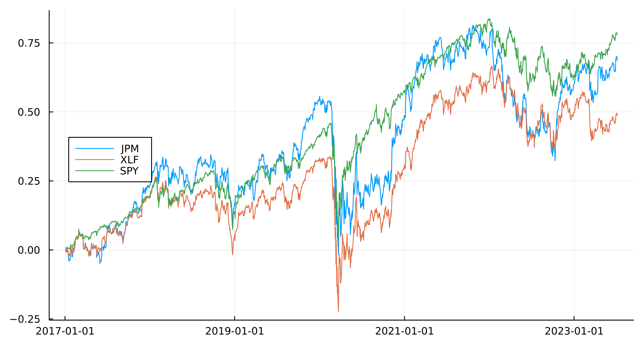
The key point is that they are moving in sync with each other. Given XLF has JPM included in it, this is expected but it also presents the opportunity to trade around any dispersion between the ETF and the individual name.
The Stat Arb Modelling Process
- https://math.stackexchange.com/questions/345773/how-the-ornstein-uhlenbeck-process-can-be-considered-as-the-continuous-time-anal
Let’s think simply about pairs trading. We have two securities that we want to trade if their prices change too much, so our variable of interest is
\[e = P_1 - P_2\]and we will enter a trade if \(e\) becomes large enough in both the positive and negative directions.
To translate that into a statistical problem we have two steps.
- Work out the difference between the two securities
- Model how the difference changes over time.
Step 1 is a simple regression of the stock vs the ETF we are trading against. Step 2 needs a bit more thought, but is still only a simple regression.
The Macro Regression - Stock vs ETF
In our data, we have the daily returns of JPM, the XLF ETF, and the SPY ETF. To work out the interdependence, it’s just a case of simple linear regression.
regModel = lm(@formula(JPM ~ XLF + SPY), modelData)
JPM ~ 1 + XLF + SPY

Coefficients:
──────────────────────────────────────────────────────────────────────────────────
                    Coef.   Std. Error       t  Pr(>|t|)   Lower 95%     Upper 95%
──────────────────────────────────────────────────────────────────────────────────
(Intercept)   0.000188758  0.000162973    1.16    0.2469  -0.0001309   0.000508417
XLF           1.35986      0.0203485     66.83    <1e-99   1.31995     1.39977
SPY          -0.363187     0.0260825    -13.92    <1e-41  -0.414345   -0.312028
──────────────────────────────────────────────────────────────────────────────────
From the slope of the model, we can see that JPM = 1.36XLF - 0.36SPY, so JPM has a \(\beta\) of 1.36 to the XLF index and a \(\beta\) of -0.36 to the SPY ETF, or general market. So each day, we can approximate JPMs return by multiplying the XLF returns and SPY returns.
This is our economic factor model, which describes from a ‘big picture’ kind of way how the stock trades vs the general market (SPY) and its sector-specific market (XLF).
What we need to do next is look at what this model doesn’t explain and try and describe that.
The Reversion Regression
Any difference around this model can be explained by the summation of the residuals over time. In the paper the sum of the residuals over time is called the ‘auxiliary process’ and this is the data behind the second regression.
plot(scatter(modelData.Date, residuals(regModel), label = "Residuals"),
       plot(modelData.Date,cumsum(residuals(regModel)),
       label = "Aux Process"),
	  layout = (2,1))

We believe the auxiliary process (cumulative sum of the residuals) can be modeled using a Ornstein-Uhlenbeck (OU) process.
An OU process is a type of differential equation that displays mean reversion behaviour. If the process falls away from its average level then it will be forced back.
\[dX = \kappa (m - X(t))dt + \sigma \mathrm{d} W\]\(\kappa\) represents how quickly the mean reversion occurs.
To fit this type of process we need to recognise that the above differential form of an OU process can be discretised to become a simple AR(1) model where the model parameters can be transformed to get the OU parameters.
We now fit the OU process onto the cumulative sum of the residuals from the first model. If the residuals have some sort of structure/pattern then this means our original model was missing some variable that explains the difference.
X = cumsum(residuals(regModel))
xDF = DataFrame(y=X[2:end], x = X[1:end-1])
arModel = lm(@formula(y~x), xDF)
y ~ 1 + x

Coefficients:
─────────────────────────────────────────────────────────────────────────────────
                  Coef.   Std. Error       t  Pr(>|t|)     Lower 95%    Upper 95%
─────────────────────────────────────────────────────────────────────────────────
(Intercept)  4.41618e-6  0.000162655    0.03    0.9783  -0.000314618  0.000323451
x            0.997147    0.00186733   534.00    <1e-99   0.993484     1.00081
─────────────────────────────────────────────────────────────────────────────────
We take these coefficients and transform them into the parameters from the paper.
varEta = var(residuals(arModel))
a, b = coef(arModel)
k = -log(b)*252
m = a/(1-b)
sigma = sqrt((varEta * 2 * k) / (1-b^2))
sigma_eq = sqrt(varEta / (1-b^2))
[m, sigma_eq]
2-element Vector{Float64}:
 0.0015477568390823153
 0.08709971423424319
So \(m\) gives us the average level and \(\sigma_{\text{eq}}\) the appropriate scale.
Now to build the mean reversion signal. We still have \(X\) as our auxiliary process which we believe is mean reverting. We now have the estimated parameters on the scale of this mean reversion so we can transform the auxiliary process by these parameters and use this to see when the process is higher or lower than the model suggests it should be.
modelData.Score = (X .- m)./sigma_eq;

plot(modelData.Date, modelData.Score, label = "s")
hline!([-1.25], label = "Long JPM, Short XLF", color = "red")
hline!([-0.5], label = "Close Long Position", color = "red", ls=:dash)

hline!([1.25], label = "Short JPM, Long XLF", color = "purple")
hline!([0.75], label = "Close Short Position", color = "purple", ls = :dash, legend=:topleft)

The red lines indicate when JPM has diverged from XLF on the negative side, i.e. we expect JPM to move higher and XLF to move lower. We enter the position if s < -1.25 (solid red line) and exit the position when s > -0.5 (dashed red line).
- Buy to open if \(s < -s_{bo}\) (< -1.25) Buy 1 JPM, sell Beta XLF
- Close long if \(s > -s_{c}\) (-0.5)
The purple line is the same but in the opposite direction.
- Sell to open if \(s > s_{so}\) (>1.25) Sell 1 JPM, buy Beta XLF
- Close short if \(s < s_{bc}\) (<0.75)
That’s the modeling part done. We model how the stock moves based on the overall market and then any differences to this we use the OU process to come up with the mean reversion parameters.
So, does it make money?
Backtesting the Stat Arb Strategy
To backtest this type of model we have to roll through time and calculate both regressions to construct the signal.
A couple of new additions too
- We shift and scale the returns when doing the macro regression.
- The auxiliary process on the last day is always 0, which makes calculating the signal simple.
paramsRes = Array{DataFrame}(undef, length(90:(nrow(modelData) - 90)))

for (j, i) in enumerate(90:(nrow(modelData) - 90))
    modelDataSub = modelData[i:(i+90), :]
    modelDataSub.JPM = (modelDataSub.JPM .- mean(modelDataSub.JPM)) ./ std(modelDataSub.JPM)
    modelDataSub.XLF = (modelDataSub.XLF .- mean(modelDataSub.XLF)) ./ std(modelDataSub.XLF)
    modelDataSub.SPY = (modelDataSub.SPY .- mean(modelDataSub.SPY)) ./ std(modelDataSub.SPY)

    macroRegr = lm(@formula(JPM ~ XLF + SPY), modelDataSub)
    auxData = cumsum(residuals(macroRegr))
    ouRegr = lm(@formula(y~x), DataFrame(x=auxData[1:end-1], y=auxData[2:end]))

    varEta = var(residuals(ouRegr))
    a, b = coef(ouRegr)
    k = -log(b)*252
    m = a/(1-b)
    sigma = sqrt((varEta * 2 * k) / (1-b^2))
    sigma_eq = sqrt(varEta / (1-b^2))


    paramsRes[j] = DataFrame(Date= modelDataSub.Date[end],
                             MacroBeta_XLF = coef(macroRegr)[2], MacroBeta_SPY = coef(macroRegr)[3], MacroAlpha = coef(macroRegr)[1],
                             VarEta = varEta, OUA = a, OUB = b, OUK = k, Sigma = sigma, SigmaEQ=sigma_eq,
                             Score = -m/sigma_eq)

end

paramsRes = vcat(paramsRes...)
last(paramsRes, 4)
4 rows × 11 columns (omitted printing of 4 columns)
| Date | MacroBeta_XLF | MacroBeta_SPY | MacroAlpha | VarEta | OUA | OUB | |
|---|---|---|---|---|---|---|---|
| Date | Float64 | Float64 | Float64 | Float64 | Float64 | Float64 | |
| 1 | 2023-06-30 | 0.974615 | -0.230273 | 1.10933e-17 | 0.331745 | 0.175358 | 0.830417 |
| 2 | 2023-07-03 | 0.96943 | -0.228741 | -5.73883e-17 | 0.331222 | 0.198176 | 0.826816 |
| 3 | 2023-07-05 | 0.971319 | -0.230438 | 2.38846e-17 | 0.335844 | 0.242754 | 0.841018 |
| 4 | 2023-07-06 | 0.974721 | -0.232765 | 5.09875e-17 | 0.331695 | 0.256579 | 0.823822 |
The benefit of doing it this way also means we can see how each \(\beta\) in the macro regression evolves.
plot(paramsRes.Date, paramsRes.MacroBeta_XLF, label = "XLF Beta")
plot!(paramsRes.Date, paramsRes.MacroBeta_SPY, label = "SPY Beta")

Good to see they are consistent in their signs and generally don’t vary a great deal.
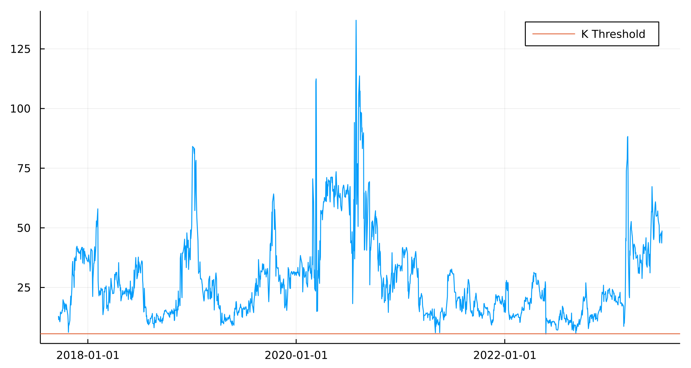
In the OU process, we are also interested in the speed of the mean reversion as we don’t want to take a position that is very slow to revert to the mean level.
kplot = plot(paramsRes.Date, paramsRes.OUK, label = :none)
kplot = hline!([252/45], label = "K Threshold")
In the paper, they suggest making sure the reversion happens with half of the estimation period. As we are using 90 days, that means the horizontal line shows when \(k\) is above this value.
Plotting the score function also shows how the model wants to go long/short the different components over time.
splot = plot(paramsRes.Date, paramsRes.Score, label = "Score")
hline!([-1.25], label = "Long JPM, Short XLF", color = "red")
hline!([-0.5], label = "Close Long Position", color = "red", ls=:dash)

hline!([1.25], label = "Short JPM, Long XLF", color = "purple")
hline!([0.75], label = "Close Short Position", color = "purple", ls = :dash)

We run through the allocation procedure and label whether we are long (+1) or short (-\(\beta\)) an amount of either the stock or ETFs.
paramsRes.JPM_Pos .= 0.0
paramsRes.XLF_Pos .= 0.0
paramsRes.SPY_Pos .= 0.0

for i in 2:nrow(paramsRes)

    if paramsRes.OUK[i] > 252/45

        if paramsRes.Score[i] >= 1.25
            paramsRes.JPM_Pos[i] = -1
            paramsRes.XLF_Pos[i] = paramsRes.MacroBeta_XLF[i]
            paramsRes.SPY_Pos[i] = paramsRes.MacroBeta_SPY[i]
        elseif paramsRes.Score[i] >= 0.75 && paramsRes.JPM_Pos[i-1] == -1
            paramsRes.JPM_Pos[i] = -1
            paramsRes.XLF_Pos[i] = paramsRes.MacroBeta_XLF[i]
            paramsRes.SPY_Pos[i] = paramsRes.MacroBeta_SPY[i]
        end

        if paramsRes.Score[i] <= -1.25
            paramsRes.JPM_Pos[i] = 1
            paramsRes.XLF_Pos[i] = -paramsRes.MacroBeta_XLF[i]
            paramsRes.SPY_Pos[i] = -paramsRes.MacroBeta_SPY[i]
        elseif paramsRes.Score[i] <= -0.5 && paramsRes.JPM_Pos[i-1] == 1
            paramsRes.JPM_Pos[i] = 1
            paramsRes.XLF_Pos[i] = -paramsRes.MacroBeta_XLF[i]
            paramsRes.SPY_Pos[i] = -paramsRes.MacroBeta_SPY[i]
        end
    end

end
To make sure we use the right price return we lead the return columns by one so that we enter the position and get the next return.
modelData = @transform(modelData, :NextJPM= lead(:JPM, 1),
                                   :NextXLF = lead(:XLF, 1),
                                   :NextSPY = lead(:SPY, 1))

paramsRes = leftjoin(paramsRes, modelData[:, [:Date, :NextJPM, :NextXLF, :NextSPY]], on=:Date)

portRes = @combine(groupby(paramsRes, :Date), :Return = :NextJPM .* :JPM_Pos .+ :NextXLF .* :XLF_Pos .+ :NextSPY .* :SPY_Pos);

plot(portRes.Date, cumsum(portRes.Return), label = "Stat Arb Return")

Sad trombone noise. This is not a great result as we’ve ended up negative over the period. However, given the paper is 15 years old it would be very rare to still be able to make money this way after everyone knows how to do it. Plus, I’ve only used one stock vs the ETF portfolio, you typically want to diversify out and use all the stocks in the ETF to be long and short multiple single names and use the ETF as a minimal hedge,
The good thing about it being a negative result means that we don’t have to start considering transaction costs or other annoying things like that.
When we break out the components of the strategy we can see that it appears to pick out the right times to short/long JPM and SPY, its the hedging with the XLF ETF that is bringing the portfolio down.
plot(paramsRes.Date, cumsum(paramsRes.NextJPM .* paramsRes.JPM_Pos), label = "JPM Component")
plot!(paramsRes.Date, cumsum(paramsRes.NextXLF .* paramsRes.XLF_Pos), label = "XLF Component")
plot!(paramsRes.Date, cumsum(paramsRes.NextSPY .* paramsRes.SPY_Pos), label = "SPY Component")
plot!(portRes.Date, cumsum(portRes.Return), label = "Stat Arb Portfolio")

So whilst naively trying to trade the stat arb portfolio is probably a loss maker, there might be some value in using the model as a signal input or overlay to another strategy.
What about if we up the frequency and look at intraday stat arb?
Intraday Stat Arb in Crypto - ETH and BTC
Crypto markets are open 24 hours a day 7 days a week and so gives that much more opportunity to build out a continuous trading model. We look back since the last year and repeat the backtesting process to see if this bares any fruit.
Once again AlpacaMarkets gives us an easy way to pull the hourly bar data for both ETH and BTC.
btcRaw = AlpacaMarkets.crypto_bars("BTC/USD", "1Hour"; startTime = now() - Year(1), limit = 10000)[1]
ethRaw = AlpacaMarkets.crypto_bars("ETH/USD", "1Hour"; startTime = now() - Year(1), limit = 10000)[1];

btc = @transform(btcRaw, :ts = DateTime.(chop.(:t)), :Ticker = "BTC")
eth = @transform(ethRaw, :ts = DateTime.(chop.(:t)), :Ticker = "ETH")

btc = btc[:, [:ts, :Ticker, :c]]
eth = eth[:, [:ts, :Ticker, :c]]

allPrices = vcat(btc, eth)
allPrices = sort(allPrices, :ts)

allPrices = @transform(groupby(allPrices, :Ticker),
                      :Return = [NaN; diff(log.(:c))]);

modelData = unstack(@select(allPrices, :ts, :Ticker, :Return), :ts, :Ticker, :Return);
modelData = @subset(modelData, .! isnan.(:ETH .+ :BTC))
Plotting out the returns we can see they are loosely related just like the stock example.
plot(modelData.ts, cumsum(modelData.BTC), label = "BTC")
plot!(modelData.ts, cumsum(modelData.ETH), label = "ETH")

We will be using BTC as the ‘index’ and see how ETH is related.
regModel = lm(@formula(ETH ~ BTC), modelData)
ETH ~ 1 + BTC

Coefficients:
─────────────────────────────────────────────────────────────────────────────
                  Coef.  Std. Error       t  Pr(>|t|)    Lower 95%  Upper 95%
─────────────────────────────────────────────────────────────────────────────
(Intercept)  7.72396e-6  3.64797e-5    0.21    0.8323  -6.37847e-5  7.92327e-5
BTC          1.115       0.00673766  165.49    <1e-99   1.10179     1.12821
─────────────────────────────────────────────────────────────────────────────
Fairly high beta for ETH and against BTC. We use a 90-hour rolling window now instead of a 90 day.
window = 90

paramsRes = Array{DataFrame}(undef, length(window:(nrow(modelData) - window)))

for (j, i) in enumerate(window:(nrow(modelData) - window))
    modelDataSub = modelData[i:(i+window), :]
    modelDataSub.ETH = (modelDataSub.ETH .- mean(modelDataSub.ETH)) ./ std(modelDataSub.ETH)
    modelDataSub.BTC = (modelDataSub.BTC .- mean(modelDataSub.BTC)) ./ std(modelDataSub.BTC)

    macroRegr = lm(@formula(ETH ~ BTC), modelDataSub)
    auxData = cumsum(residuals(macroRegr))
    ouRegr = lm(@formula(y~x), DataFrame(x=auxData[1:end-1], y=auxData[2:end]))
    varEta = var(residuals(ouRegr))
    a, b = coef(ouRegr)
    k = -log(b)/((1/24)/252)
    m = a/(1-b)
    sigma = sqrt((varEta * 2 * k) / (1-b^2))
    sigma_eq = sqrt(varEta / (1-b^2))


    paramsRes[j] = DataFrame(ts= modelDataSub.ts[end], MacroBeta = coef(macroRegr)[2], MacroAlpha = coef(macroRegr)[1],
                             VarEta = varEta, OUA = a, OUB = b, OUK = k, Sigma = sigma, SigmaEQ=sigma_eq,
                             Score = -m/sigma_eq)

end

paramsRes = vcat(paramsRes...)
Again, looking at \(\beta\) overtime we see there has been a sudden shift
plot(plot(paramsRes.ts, paramsRes.MacroBeta, label = "Macro Beta", legend = :left),
     plot(paramsRes.ts, paramsRes.OUK, label = "K"), layout = (2,1))

Interesting that there has been a big change in \(\beta\) between ETH and BTC recently that has suddenly reverted. Ok, onto the backtesting again.
paramsRes.ETH_Pos .= 0.0
paramsRes.BTC_Pos .= 0.0

for i in 2:nrow(paramsRes)

    if paramsRes.OUK[i] > (252/(1/24)/45)

        if paramsRes.Score[i] >= 1.25
            paramsRes.ETH_Pos[i] = -1
            paramsRes.BTC_Pos[i] = paramsRes.MacroBeta[i]
        elseif paramsRes.Score[i] >= 0.75 && paramsRes.ETH_Pos[i-1] == -1
            paramsRes.ETH_Pos[i] = -1
            paramsRes.BTC_Pos[i] = paramsRes.MacroBeta[i]
        end

        if paramsRes.Score[i] <= -1.25
            paramsRes.ETH_Pos[i] = 1
            paramsRes.BTC_Pos[i] = -paramsRes.MacroBeta[i]
        elseif paramsRes.Score[i] <= -0.5 && paramsRes.ETH_Pos[i-1] == 1
            paramsRes.ETH_Pos[i] = 1
            paramsRes.BTC_Pos[i] = -paramsRes.MacroBeta[i]
        end
    end

end


modelData = @transform(modelData, :NextETH= lead(:ETH, 1), :NextBTC = lead(:BTC, 1))

paramsRes = leftjoin(paramsRes, modelData[:, [:ts, :NextETH, :NextBTC]], on=:ts)

portRes = @combine(groupby(paramsRes, :ts), :Return = :NextETH .* :ETH_Pos .+ :NextBTC .* :BTC_Pos);

plot(portRes.ts, cumsum(portRes.Return))

This looks slightly better. At least it is positive at the end of the testing period.
plot(paramsRes.ts, cumsum(paramsRes.NextETH .* paramsRes.ETH_Pos), label = "ETH Component")
plot!(paramsRes.ts, cumsum(paramsRes.NextBTC .* paramsRes.BTC_Pos), label = "BTC Component")
plot!(portRes.ts, cumsum(portRes.Return), label = "Stat Arb Portfolio", legend=:topleft)

Again, the components of the portfolio seem to be ok in the ETH case but generally, this is from the overall long bias. Unlike the JPM/XLF example, there isn’t much more diversification we can add anything that might help. We could add in more crypto assets, or an equity/gold angle, but it becomes more of an asset class arb than something truly statistical.
Conclusion
The original paper is one of those that all quants get recommended to read and statistical arbitrage is a concept that you probably understand in theory but practically doing is another question. Hopefully, this blog post gets you up to speed with the basic concepts and how to implement them. It can be boiled down to two steps.
- Model as much as you can with a simple regression
- Model what’s left over as an OU process.
It can work with both high-frequency and low-frequency data, so have a look at different combinations or assets and see if you have more luck then I did backtesting.
If you do end up seeing something positive, make sure you are backtesting properly!