Exploring Causal Regularisation

A good prediction model isn’t necessarily a good causal model. You could be missing a key variable in your dataset that is driving the underlying behavior so you end up with a good predictive model but not the correct explanation as to why things behave that way. Taking a causal approach is a tougher problem and needs an understanding of whether we have access to the right variables or we are making the right link between variables and an outcome. Causal regularisation is a method that uses machine learning techniques (regularisation!) to try and produce models that can be interpreted causally.

Enjoy these types of posts? Then you should sign up for my newsletter.

Regularisation is normally taught as a method to reduce overfitting, you have a big model and you make it smaller by shrinking some of the factors. Work by Janzing (papers below) argues that this can help produce better causal models too and in this blog post I will work through two papers to try and understand the process better.

I’ll work off two main papers for causal regularisation:

In truth, I am working backward. I first encountered causal regularisation in Better AB testing via Causal Regularisation where it uses causal regularisation to produce better estimates by combining a biased and an unbiased dataset. I want to take a step back and understand casual regularisation from the original papers. Using free data from the UCI Machine Learning Repository we can attempt to replicate the methods from the papers and see how causal regularisation works to produce better causal models.

As ever, I’m in Julia (1.9), so fire up that notebook and follow along.

using CSV, DataFrames, DataFramesMeta
using Plots
using GLM, Statistics

Wine Tasting Data

The wine-quality dataset from the UCI repository provides measurements of the chemical properties of wine and a quality rating from someone drinking the wine. It’s a simple CSV file that you can download (winequality) and load with minimal data wrangling needed.

We will be working with the red wine data set as that’s what both Janzing papers use.

rawData = CSV.read("wine+quality/winequality-red.csv", DataFrame)
first(rawData)

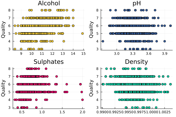
APD! Always Plotting the Data to make sure the values are something you expect. Sometimes you need a visual confirmation that things line up with what you believe.

plot(scatter(rawData.alcohol, rawData.quality, title = "Alcohol", label = :none, color="#eac435"),
     scatter(rawData.pH, rawData.quality, title = "pH", label = :none, color="#345995"),
     scatter(rawData.sulphates, rawData.quality, title= "Sulphates", label = :none, color="#E40066"),
     scatter(rawData.density, rawData.quality, title = "Density", label = :none, color="#03CEA4"), ylabel = "Quality")

Wine quality variable relationships

By choosing four of the variables randomly we can see that some are correlated with quality and some are not.

A loose goal is to come up with a causal model that can explain the quality of the wine using the provided factors. We will change the data slightly to highlight how causal regularisation helps, but for now, let’s start with the simple OLS model.

In the paper they normalise the variables to be unit variance, so we divide by the standard deviation. We then model the quality of the wine using all the available variables.

vars = names(rawData, Not(:quality))

cleanData = deepcopy(rawData)

for var in filter(!isequal("White"), vars)
    cleanData[!, var] = cleanData[!, var] ./ std(cleanData[!, var])
end

cleanData[!, :quality] .= Float64.(cleanData[!, :quality])

ols = lm(term(:quality) ~ sum(term.(Symbol.(vars))), cleanData)

StatsModels.TableRegressionModel{LinearModel{GLM.LmResp{Vector{Float64}}, GLM.DensePredChol{Float64, LinearAlgebra.CholeskyPivoted{Float64, Matrix{Float64}, Vector{Int64}}}}, Matrix{Float64}}

quality ~ 1 + fixed acidity + volatile acidity + citric acid + residual sugar + chlorides + free sulfur dioxide + total sulfur dioxide + density + pH + sulphates + alcohol

Coefficients:
────────────────────────────────────────────────────────────────────────────────────────
                           Coef.  Std. Error      t  Pr(>|t|)     Lower 95%    Upper 95%
────────────────────────────────────────────────────────────────────────────────────────
(Intercept)           21.9652     21.1946      1.04    0.3002  -19.6071      63.5375
fixed acidity          0.043511    0.0451788   0.96    0.3357   -0.0451055    0.132127
volatile acidity      -0.194027    0.0216844  -8.95    <1e-18   -0.23656     -0.151494
citric acid           -0.0355637   0.0286701  -1.24    0.2150   -0.0917989    0.0206716
residual sugar         0.0230259   0.0211519   1.09    0.2765   -0.0184626    0.0645145
chlorides             -0.088211    0.0197337  -4.47    <1e-05   -0.126918    -0.0495041
free sulfur dioxide    0.0456202   0.0227121   2.01    0.0447    0.00107145   0.090169
total sulfur dioxide  -0.107389    0.0239718  -4.48    <1e-05   -0.154409    -0.0603698
density               -0.0337477   0.0408289  -0.83    0.4086   -0.113832     0.0463365
pH                    -0.0638624   0.02958    -2.16    0.0310   -0.121883    -0.00584239
sulphates              0.155325    0.019381    8.01    <1e-14    0.11731      0.19334
alcohol                0.294335    0.0282227  10.43    <1e-23    0.238977     0.349693
────────────────────────────────────────────────────────────────────────────────────────

The dominant factor is the alcohol amount which is the strongest variable in predicting the quality, i.e. higher quality has a higher alcohol content. We also note that 5 out of the 12 variables are deemed insignificant at the 5% level. We save these parameters and then look at the regression without the alcohol variable.

olsParams = DataFrame(Dict(zip(vars, coef(ols)[2:end])))
olsParams[!, :Model] .= "OLS"
olsParams

1×12 DataFrame

Row	alcohol	chlorides	citric acid	density	fixed acidity	free sulfur dioxide	pH	residual sugar	sulphates	total sulfur dioxide	volatile acidity	Model
	Float64	Float64	Float64	Float64	Float64	Float64	Float64	Float64	Float64	Float64	Float64	String
1	0.294335	-0.088211	-0.0355637	-0.0337477	0.043511	0.0456202	-0.0638624	0.0230259	0.155325	-0.107389	-0.194027	OLS

cleanDataConfounded = select(cleanData, Not(:alcohol))
vars = names(cleanDataConfounded, Not(:quality))

confoundOLS = lm(term(:quality) ~ sum(term.(Symbol.(vars))), cleanDataConfounded)

StatsModels.TableRegressionModel{LinearModel{GLM.LmResp{Vector{Float64}}, GLM.DensePredChol{Float64, LinearAlgebra.CholeskyPivoted{Float64, Matrix{Float64}, Vector{Int64}}}}, Matrix{Float64}}

quality ~ 1 + fixed acidity + volatile acidity + citric acid + residual sugar + chlorides + free sulfur dioxide + total sulfur dioxide + density + pH + sulphates

Coefficients:
───────────────────────────────────────────────────────────────────────────────────────────
                             Coef.  Std. Error       t  Pr(>|t|)     Lower 95%    Upper 95%
───────────────────────────────────────────────────────────────────────────────────────────
(Intercept)           189.679       14.2665      13.30    <1e-37  161.696       217.662
fixed acidity           0.299551     0.0391918    7.64    <1e-13    0.222678      0.376424
volatile acidity       -0.176182     0.0223382   -7.89    <1e-14   -0.219997     -0.132366
citric acid             0.00912711   0.0292941    0.31    0.7554   -0.0483321     0.0665863
residual sugar          0.133781     0.0189031    7.08    <1e-11    0.0967031     0.170858
chlorides              -0.107215     0.0203052   -5.28    <1e-06   -0.147043     -0.0673877
free sulfur dioxide     0.0394281    0.023462     1.68    0.0931   -0.00659172    0.0854479
total sulfur dioxide   -0.128248     0.0246854   -5.20    <1e-06   -0.176668     -0.0798287
density                -0.355576     0.0276265  -12.87    <1e-35   -0.409765     -0.301388
pH                      0.0965662    0.0261087    3.70    0.0002    0.0453551     0.147777
sulphates               0.213697     0.0191745   11.14    <1e-27    0.176087      0.251307
───────────────────────────────────────────────────────────────────────────────────────────

citric acid and free sulfur dioxide are now the only insignificant variables, the rest are believed to contribute to the quality. This means we are experiencing confounding as alcohol is the better explainer but the effect of alcohol is now hiding behind these other variables.

Confounding - When a variable influences other variables and the outcome at the same time leading to an incorrect view on the correlation between the variables and outcomes.

This regression after dropping the alcohol variable is incorrect and provides the wrong causal conclusion. So can we do better and get closer to the true regression coefficients using some regularisation methods?

For now, we save these incorrect parameters and explore the causal regularisation methods.

olsParamsConf = DataFrame(Dict(zip(vars, coef(confoundOLS)[2:end])))
olsParamsConf[!, :Model] .= "OLS No Alcohol"
olsParamsConf[!, :alcohol] .= NaN

olsParamsConf

1×12 DataFrame

Row	chlorides	citric acid	density	fixed acidity	free sulfur dioxide	pH	residual sugar	sulphates	total sulfur dioxide	volatile acidity	Model	alcohol
	Float64	Float64	Float64	Float64	Float64	Float64	Float64	Float64	Float64	Float64	String	Float64
1	-0.107215	0.00912711	-0.355576	0.299551	0.0394281	0.0965662	0.133781	0.213697	-0.128248	-0.176182	OLS No Alcohol	NaN

Regularisation and Regression

Some maths. Regression is taking our variables $X$ and finding the parameters $a$ that get us closest to $Y$.

\[Y = a X\]

$X$ is a matrix, and $a$ is a vector. When we fit this to some data, the values of $a$ are free to converge to any value they want, so long as it gets close to the outcome variable. This means we are minimising the difference between $Y$ and $X$

\[||(Y - a X)|| ^2.\]

Regularisation is the act of restricting the values $a$ can take.

For example, we can make the sum of all the $a$’s equal to a constant (L_1 regularisation), or the sum of the square of the $a$ values equal a constant (L_2 regularisation). In simpler terms, if we want to increase the coefficient of one parameter, we need to reduce the parameter of a different term. Think of there being a finite amount of mass that we can allocate to the parameters, they can’t take on whatever value they like, but instead need to regulate amongst themselves. This helps reduce overfitting as it constrains how much influence a parameter can have and the final result should converge to a model that doesn’t overfit.

In ridge regression we are minimising the $L_2$ norm, so restricting the sum of the square of the $a$’s and at the same time minimising the original OLS regression.

\[||(Y - a X)|| ^2 - \lambda || a || ^2.\]

So we can see how regularisation is an additional component of OLS regression. $\lambda$ is a hyperparameter that is just a number and controls how much restriction we place on the $a$ values.

To do ridge regression in Julia I’ll be leaning on the MLJ.jl framework and using that to build out the learning machines.

using MLJ

@load RidgeRegressor pkg=MLJLinearModels

We will take the confounded dataset (so the data where the alcohol column is deleted), partition it into train and test sets, and get started with some regularisation.

y, X = unpack(cleanDataConfounded, ==(:quality); rng=123);

train, test = partition(eachindex(y), 0.7, shuffle=true)

mdl = MLJLinearModels.RidgeRegressor()

RidgeRegressor(
  lambda = 1.0, 
  fit_intercept = true, 
  penalize_intercept = false, 
  scale_penalty_with_samples = true, 
  solver = nothing)

Can see the hyperparameter lambda is initialised to 1.

Basic Ridge Regression

We want to know the optimal $\lambda$ value so will use cross-validation to train the model on one set of data and verify on a hold-out set before repeating. This is all simple in MLJ.jl, we define a grid of penalisations between 0 and 1 and fit the regression using cross-validation across the different lambdas. We are optimising for the best $R^2$ value.

lambda_range = range(mdl, :lambda, lower = 0, upper = 1)

lmTuneModel = TunedModel(model=mdl,
                          resampling = CV(nfolds=6, shuffle=true),
                          tuning = Grid(resolution=200),
                          range = [lambda_range],
                          measures=[rsq]);

lmTunedMachine = machine(lmTuneModel, X, y);

fit!(lmTunedMachine, rows=train, verbosity=0)
report(lmTunedMachine).best_model

RidgeRegressor(
  lambda = 0.020100502512562814, 
  fit_intercept = true, 
  penalize_intercept = false, 
  scale_penalty_with_samples = true, 
  solver = nothing)

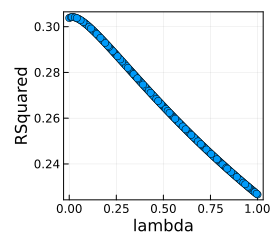
The best value of $\lambda$ is 0.0201. When we plot the $R^2$ vs the $\lambda$ values there isn’t that much of a change just a minor inflection around the small ones.

plot(lmTunedMachine)

R2 and lambda for basic ridge regression

Let’s save those parameters. This will be our basic ridge regression result that the other technique builds off.

res = fitted_params(lmTunedMachine).best_fitted_params.coefs

ridgeParams = DataFrame(res)
ridgeParams = hcat(ridgeParams, DataFrame(Model = "Ridge", alcohol=NaN))
ridgeParams

1×12 DataFrame

Row	fixed acidity	volatile acidity	citric acid	residual sugar	chlorides	free sulfur dioxide	total sulfur dioxide	density	pH	sulphates	Model	alcohol
	Float64	Float64	Float64	Float64	Float64	Float64	Float64	Float64	Float64	Float64	String	Float64
1	0.190892	-0.157286	0.0410523	0.117846	-0.142458	0.0374597	-0.153419	-0.29919	0.0375852	0.232461	Ridge	NaN

Implementing Causal Regularisation

The main result from the paper is that we first need to estimate the confounding effect $\beta$ and then choose a penalisation factor $\lambda$ that satisfies

\[(1-\beta) || a || ^ 2\]

So the $L_2$ norm of the ridge parameters can only be so much. In the 2nd paper, they estimate $\beta$ to be 0.8. For us, we can use the above grid search, calculate the norm of the parameters, and find which ones satisfy those criteria.

So iterate through the above results of the grid search, and calculate the L2 norm of the parameters.

mdls = report(lmTunedMachine).history

l = zeros(length(mdls))
a = zeros(length(mdls))

for (i, mdl) in enumerate(mdls)
    l[i] = mdl.model.lambda
    a[i] = sum(map( x-> x[2], fitted_params(fit!(machine(mdl.model, X, y))).coefs) .^2)
end

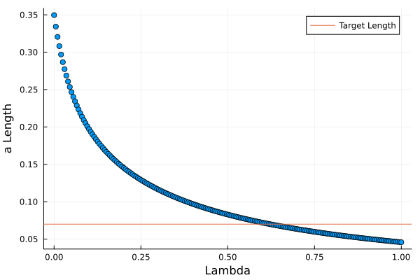
Plotting the results gives us a visual idea of how the penalisation works. Larger values of $\lambda$ mean the model parameters are more and more restricted.

inds = sortperm(l)
l = l[inds]
a = a[inds]

mdlsSorted = report(lmTunedMachine).history[inds]

scatter(l, a, label = :none)
hline!([(1-0.8) * sum(coef(confoundOLS)[2:end] .^ 2)], label = "Target Length", xlabel = "Lambda", ylabel = "a Length")

R2 and lambda for basic ridge regression with target length

We search the lengths for the one closest to the target length and save those parameters.

targetLength = (1-0.8) * sum(coef(confoundOLS)[2:end] .^ 2)
ind = findfirst(x-> x < targetLength, a)

res = fitted_params(fit!(machine(mdlsSorted[ind].model, X, y))).coefs

finalParams = DataFrame(res)
finalParams = hcat(finalParams, DataFrame(Model = "With Beta", alcohol=NaN))
finalParams

1×12 DataFrame

Row	fixed acidity	volatile acidity	citric acid	residual sugar	chlorides	free sulfur dioxide	total sulfur dioxide	density	pH	sulphates	Model	alcohol
	Float64	Float64	Float64	Float64	Float64	Float64	Float64	Float64	Float64	Float64	String	Float64
1	0.0521908	-0.139099	0.0598797	0.0377729	-0.0786037	0.00654776	-0.0856938	-0.124057	0.00682623	0.11735	With Beta	NaN

What if we don’t want to calculate the confounding effect?

Now the code to calculate $\beta$ isn’t the easiest or straightforward to implement (hence why I took their estimate). Instead, we could take the approach from Better AB Testing via Causal Regularisation and use the test set to optimise the penalisation parameter $\lambda$ and then use that value when training the model on the train set.

Applying this method to the wine dataset isn’t a true replication of their paper, as their test and train data sets are instead two data sets, one with bias and one without like you might observe from an AB test. So it’s more of a demonstration of the method rather than a direct comparison to the Janzing method.

Again, MLJ makes this simple, we just fit the machine using the test rows to produce the best-fitting model.

lambda_range = range(mdl, :lambda, lower = 0, upper = 1)

lmTuneModel = TunedModel(model=mdl,
                          resampling = CV(nfolds=6, shuffle=true),
                          tuning = Grid(resolution=200),
                          range = [lambda_range],
                          measures=[rsq]);

lmTunedMachine = machine(lmTuneModel, X, y);

fit!(lmTunedMachine, rows=test, verbosity=0)
plot(lmTunedMachine)

R2 and lambda for basic ridge regression on the test set

report(lmTunedMachine).best_model

RidgeRegressor(
  lambda = 0.010050251256281407, 
  fit_intercept = true, 
  penalize_intercept = false, 
  scale_penalty_with_samples = true, 
  solver = nothing)

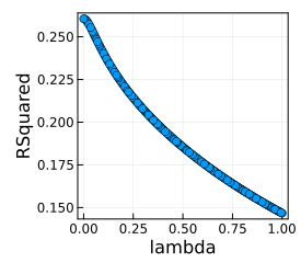
Our best $\lambda$ is 0.01 so we retrain the same machine, this time using the training rows.

res2 = fit!(machine(report(lmTunedMachine).best_model, X, y), rows=train)

Again saving these parameters down leaves us with three methods and three sets of parameters.

finalParams2 = DataFrame(fitted_params(res2).coefs)
finalParams2 = hcat(finalParams2, DataFrame(Model = "No Beta", alcohol=NaN))

allParams = vcat([olsParams, olsParamsConf, ridgeParams, finalParams, finalParams2]...)
allParams

5×12 DataFrame

Row	alcohol	chlorides	citric acid	density	fixed acidity	free sulfur dioxide	pH	residual sugar	sulphates	total sulfur dioxide	volatile acidity	Model
	Float64	Float64	Float64	Float64	Float64	Float64	Float64	Float64	Float64	Float64	Float64	String
1	0.294335	-0.088211	-0.0355637	-0.0337477	0.043511	0.0456202	-0.0638624	0.0230259	0.155325	-0.107389	-0.194027	OLS
2	NaN	-0.107215	0.00912711	-0.355576	0.299551	0.0394281	0.0965662	0.133781	0.213697	-0.128248	-0.176182	OLS No Alcohol
3	NaN	-0.142458	0.0410523	-0.29919	0.190892	0.0374597	0.0375852	0.117846	0.232461	-0.153419	-0.157286	Ridge
4	NaN	-0.0786037	0.0598797	-0.124057	0.0521908	0.00654776	0.00682623	0.0377729	0.11735	-0.0856938	-0.139099	With Beta
5	NaN	-0.141766	0.031528	-0.323596	0.222812	0.03869	0.048907	0.127026	0.23961	-0.153488	-0.157603	No Beta

What method has done the best at uncovering the confounded relationship?

Relative Squared Error

We have our different estimates of the parameters of the model, we now want to compare these to the ‘true’ unconfounded variables and see whether we have recovered the correct variables. To do this we calculate the square difference and normalise by the overall $L_2$ norm of the parameters.

In practice, this just means we are comparing how far the fitted parameters are away from the true (unconfounded) model parameters.

allParamsLong = stack(allParams, Not(:Model))
trueParams = select(@subset(allParamsLong, :Model .== "OLS"), Not(:Model))
rename!(trueParams, ["variable", "truth"])
allParamsLong = leftjoin(allParamsLong, trueParams, on = :variable)
errorRes = @combine(groupby(@subset(allParamsLong, :variable .!= "alcohol"), :Model), 
         :a = sum((:truth .- :value) .^2),
         :a2 = sum(:value .^ 2))
errorRes = @transform(errorRes, :e = :a ./ :a2)
sort(errorRes, :e)

5×4 DataFrame

Row	Model	a	a2	e
	String	Float64	Float64	Float64
1	OLS	0.0	0.0920729	0.0
2	With Beta	0.0291038	0.0698576	0.416616
3	Ridge	0.129761	0.266952	0.486085
4	No Beta	0.157667	0.301286	0.523314
5	OLS No Alcohol	0.213692	0.349675	0.611116

Using the $\beta$ estimation method gives the best model (smallest $e$), which lines up with the paper and the magnitude of error is also inline with the paper (they had 0.35 and 0.45 for Lasoo/ridge regression respectively). The ridge regression and no beta method also improved on the naive OLS approach, so that indicates that there is some improvement from using these methods. The No Beta method is not a faithful reproduction of the Better AB testing paper because it requires the ‘test’ dataset to be an AB test scenario, which we don’t have from the above, so that might explain why the values don’t quite line up.

All methods improve on the naive ‘OLS No Alcohol’ parameters though, which shows this approach to causal regularisation can uncover better models if you have underlying confounding in your data.

Summary

We are always stuck with the data we are given and most of the time can’t collect more to try and uncover more relationships. Causal regularisation gives us a chance to use normal machine learning techniques to build better causal relationships by guiding what the regularisation parameters should be and using that to restrict the overall parameters. When we can estimate the expected confounding value $\beta$ we get the best results, but regular ridge regression and the Webster-Westray method also provide an improvement on just doing a naive regression. So whilst overfitting is the main driver for doing regularisation it also brings with it some causal benefits and lets you understand true relationships between variables in a truer sense.

Another Causal Post

I’ve written about causal analysis techniques before with Double Machine Learning - An Easy Introduction. This is another way of building causal models.