Currency Hedging and Principal Component Analysis
Principal component analysis (PCA) reduces a dataset to its main components. When we apply it to a dataset of different currencies it helps us understand how each currency drives the overall portfolio and what currency might be a common factor.
Enjoy these types of posts? Then you should sign up for my newsletter.
This post was inspired by a problem on the r/quant subreddit where someone posted their interview/take-home question.
A client is considering using SGD to (proxy) hedge their exposure to a basket of other Asian currencies. Is this likely to be effective? What analysis could you produce that would help inform their decision? The client is a US Corporate. The client is exposed to medium-term changes (say monthly) in the currency. The client has equal (USD equivalent) revenues in each Asian currency. We are not considering hedging costs for this analysis (spot-only component). The data for daily close spot values against USD for each pair is provided. Which currency pairs will it work better for? Would it work for an equally weighted currency portfolio? Would another (single) currency work better? Which correlations should we consider and how reliable are these?
This is an interesting question and not too dissimilar to the occasional question I answer in my day job. So I thought I’d run through how I might answer it.
Getting FX Data
First, we need to get some data and I’ll be using Alphavantage to pull daily closing prices of the different currencies. I’ll calculate the log returns and save the data to cache it for future use. Plus AlphaVantage only lets you make 25 calls a day, so each time I mucked up I got locked out for the day - delaying the analysis. We have to start from 2014 as this is the earliest common date across all currencies.
function _pull_data(ccy)
    println(ccy)
    res = AlphaVantage.fx_daily("USD", ccy, outputsize="full", datatype="csv")
    res = DataFrame(Dict(:Date=>Date.(res[1][:, 1]), :c=>Float64.(res[1][:,5]), :ccy => ccy));
    res = sort(res, :Date)
    res = @transform(res, :LogReturn = [0; diff(log.(:c))])
    res
end

function pull_data(ccy)
    if isfile("$ccy.csv")
        res = CSV.read("$ccy.csv", DataFrame)
    else
        res = _pull_data(ccy)
        CSV.write("$ccy.csv", res)
    end
    res
end

ccys = ["JPY", "CNH", "SGD", "THB", "HKD", "KRW", "TWD"]
res = vcat(pull_data.(ccys)...);
res = sort(res, :Date)
res = @transform(groupby(res, :ccy), :LogReturn = [0; diff(log.(:c))])
res = @subset(res, :Date .>= Date("2014-11-24"))
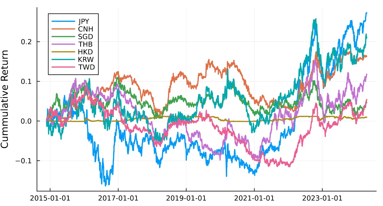
Like all good blog posts, let’s start with the plot of the cumulative returns. Only HKD stands out as something different given its peg to USD.
p = plot(ylabel = "Cummulative Return")
for ccy in ccys
    plot!(p, res[res.ccy .== ccy, :].Date, cumsum(res[res.ccy .== ccy, :].LogReturn), label = ccy, lw = 2)
end
p
According to the problem, our client is long equal amounts of these Asian currencies, so it makes sense to calculate the market returns by taking the average return each day.
market = @combine(groupby(res, :Date), :LogReturn = mean(:LogReturn))
market[!, :ccy] .= "Market"
market[!, :c] .= NaN;
Which we add to the original plot.
p = plot!(p, market.Date, cumsum(market.LogReturn)
    label = "Market", color = "black", lw  = 2)
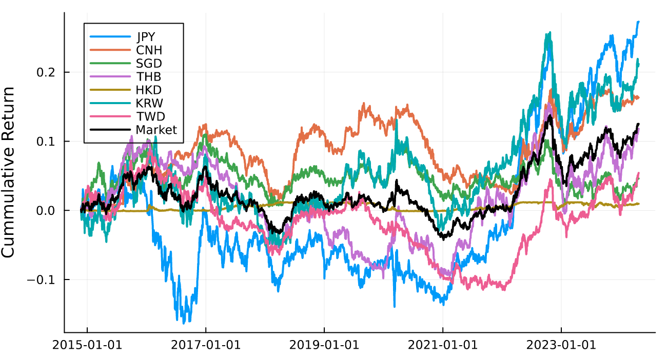
The client thinks that hedging with SGD alone is enough to protect against the overall market returns. We can see from the graph that this probably isn’t the case. But how do we recommend a better approach?
First, we will start with the correlation in returns between the different currencies. This will shed some light on how linked they are and is also simple to explain to the client.
cr = cor(Matrix(modelData[:, [:JPY, :CNH, :SGD, :THB, :HKD, :KRW, :TWD]]))
heatmap(ccys, ccys, cr .> 0.5)
We use a heat-map, but only highlight when two currencies have a correlation > 0.5, otherwise it’s a bit of a psychedelic nightmare.
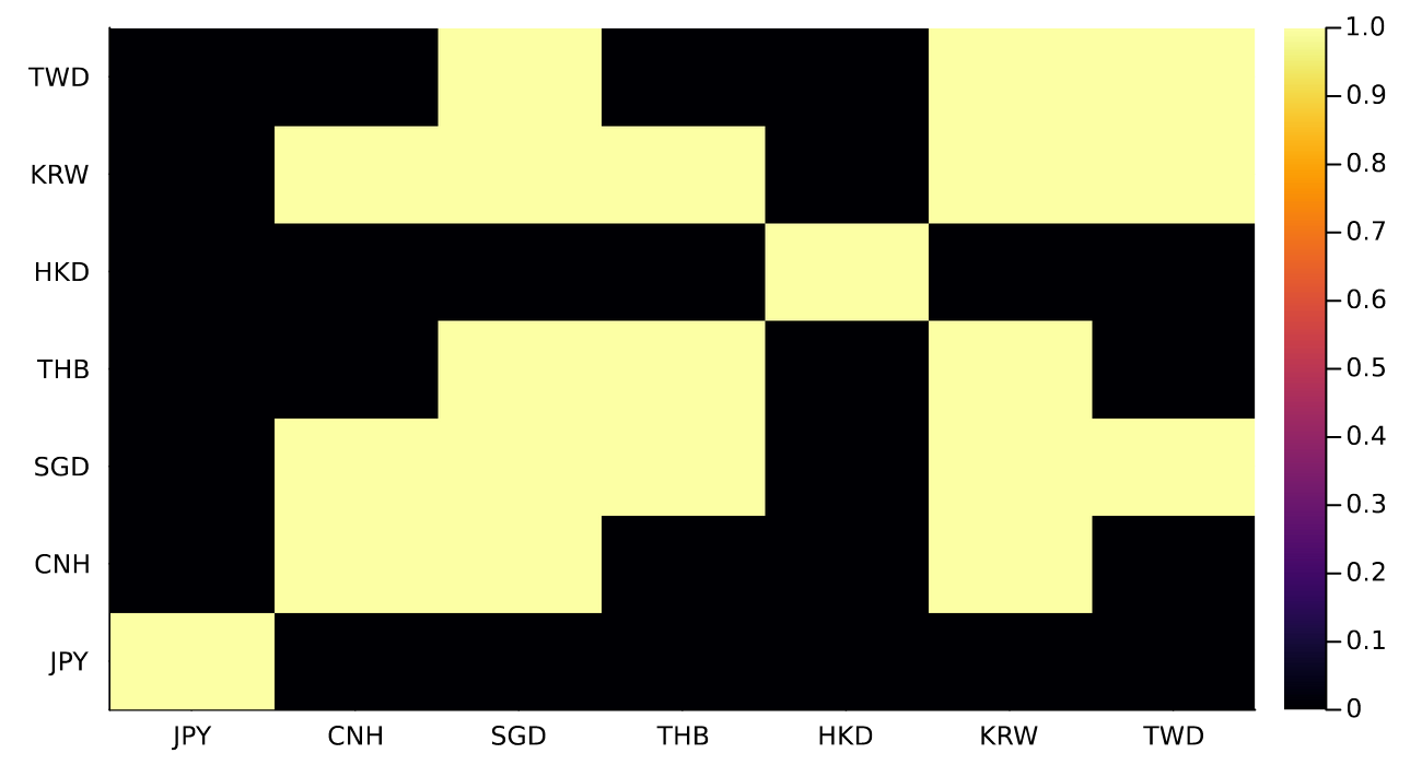
We can see that HKD has a low correlation with most, KRW and SGD have a high correlation between each other and KRW has a high correlation with the majority of these currencies. However, we will use the covariance matrix to analyse the best hedging portfolio rather than the correlation matrix.
Principal Component Analysis
Principal component analysis (or PCA) is a tool that tries to find a common basis of variation in a matrix. It’s about transforming the data into uncorrelated components through linear algebra.
For this we are using the covariance matrix, so now the diagonals are the individual price series variances and the off-diagonals are the covariances between two currencies. If this were a different problem we might rescale the returns so they all had the same volatility but this would mean applying leverage, which our hypothetical customer probably wouldn’t be up for it.
We pull out the covariance matrix
modelData = dropmissing(unstack(res, :Date, :ccy, :LogReturn))
cm = cov(Matrix(modelData[:, [:JPY, :CNH, :SGD, :THB, :HKD, :KRW, :TWD]]))
The MultivariateStats.jl package has the functions for doing PCA and
the appropriate functions for pulling out the right data after fitting the
PCA model.
pcaRes = fit(PCA, cm; maxoutdim=3)
Firstly the weights of all the currencies for the three principal components.
| PC1 Weights | PC2 Weights | PC3 Weights | |
|---|---|---|---|
| JPY | 4.96845E-06 | 9.11362E-06 | -2.98467E-07 |
| CNH | 2.11372E-06 | -1.1987E-06 | -4.78571E-08 |
| SGD | 3.35545E-06 | -5.17405E-07 | -1.00414E-07 |
| THB | 3.21579E-06 | -7.50513E-07 | 3.05907E-06 |
| HKD | 4.21256E-08 | -7.74387E-08 | -1.84514E-08 |
| KRW | 7.67389E-06 | -4.39207E-06 | -8.40943E-07 |
| TWD | 2.42907E-06 | -2.01299E-06 | -6.01965E-07 |
- PC1 shows the weights for each currency but is unnormalised. The key thing we can see here is that HKD is magnitudes smaller than the others.
- PC2 is long JPY and short all the others
- PC3 is long THB and short all the others
Then the explained variance of the three components.
| PC1 | PC2 | PC3 | |
|---|---|---|---|
| Eigenvalues | 1.15544e-10 | 1.08674e-10 | 1.05292e-11 |
| Variance explained | 0.47267 | 0.444567 | 0.0430731 |
| Cumulative variance | 0.47267 | 0.917237 | 0.96031 |
The first component can explain 49% of the variance and then including the second component 91% of the variance, with the final component making up 5% to take it to 96% in total. This means that this dataset can be broken down quite nicely into the two principal components and this explains most of the variation.
The first principal component is commonly called the ‘market’ portfolio and represents the overall combined market dynamics of the portfolio. The next portfolio (using the 2nd PC weights) is uncorrelated to the market and thus more diversified to the overall market.
In our problem then we can see that we are trying to come up with a representation of the market and use that to decide how to hedge out our currencies. So the first principal component is the most relevant.
We take these principal component weights and join them to the original dataframe to start exploring what the market portfolio looks like.
evFrame = DataFrame(Dict(:ccy => String.([:JPY, :CNH, :SGD, :THB, :HKD, :KRW, :TWD]),
          :ev1 => eigvecs(pcaRes)[:,1],
          :ev2 => eigvecs(pcaRes)[:,2]))
sort!(evFrame, :ev1)

res = leftjoin(res, dropmissing(evFrame), on = :ccy)

evFrame = sort(evFrame, :ev1);
Then plotting the weights by currency pair
bar(evFrame.ccy, evFrame.ev1 ./ sum(evFrame.ev1), label = "Eigen Weights")
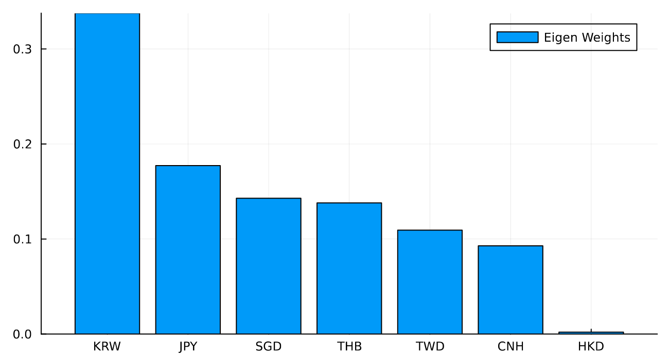
These are the weights of the different currencies of the first eigen portfolio. This combination of currencies is what we would recommend if the client was exposed to a similar basket. The key points:
- The client is long these currencies through their business
- They short this portfolio and thus are market-neutral
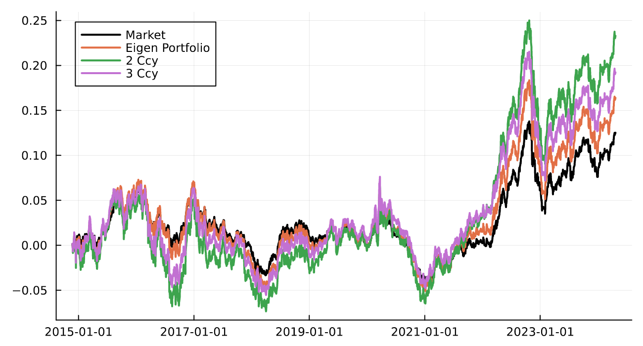
We now calculate the returns of the eigen portfolios, the portfolio that only uses the largest 2 (and 3) weights.
evPortfolios = @combine(groupby(res, :Date),
         :ReturnEV1 = sum(:LogReturn .* :ev1) ./ sum(:ev1),
         :ReturnEV2 = sum(:LogReturn .* :ev2) ./ sum(:ev2));

ccy2Portfolio = @combine(groupby(res[in.(res.ccy, Ref(["KRW", "JPY"])), :], :Date),
         :Return2Ccy = sum(:LogReturn .* :ev1) ./ sum(:ev1));

ccy3Portfolio = @combine(groupby(res[in.(res.ccy, Ref(["KRW", "JPY", "SGD"])), :], :Date),
         :Return3Ccy = sum(:LogReturn .* :ev1) ./ sum(:ev1));
And plotting these returns
plot(market.Date, cumsum(market.LogReturn), label = "Market", color = "black", lw = 2)
plot!(evPortfolios.Date,  cumsum(evPortfolios.ReturnEV1), label = "Eigen Portfolio", lw = 2)
plot!(ccy2Portfolio.Date,  cumsum(ccy2Portfolio.Return2Ccy), label = "2 Ccy", lw =2)
plot!(ccy3Portfolio.Date,  cumsum(ccy3Portfolio.Return3Ccy), label = "3 Ccy", lw = 2)
Then finally, looking at the correlation between these portfolios
| Market Return | Market Eigen Portfolio | 2nd Eigen Portfolio | KRW + JPY | KRW + JPY + SGD | |
|---|---|---|---|---|---|
| Market Return | 1.0 | 0.99 | 0.01 | 0.93 | 0.95 |
| Market Eigen Portfolio | 0.99 | 1.0 | 0.01 | 0.97 | 0.98 |
| 2nd Eigen Portfolio | 0.01 | 0.01 | 1.0 | 0.11 | 0.08 |
| KRW + JPY | 0.93 | 0.97 | 0.11 | 1.0 | 0.99 |
| KRW + JPY + SGD | 0.95 | 0.99 | 0.08 | 0.99 | 1.0 |
- The Eigen Portfolio 1 is most correlated with the equal-weighted portfolio.
- With just KRW and JPY you get to a 93% correlation with the market.
- KRW, JPY and SGD gets you to a 95% with the market.
As expected Eigen portfolio 2 is the most uncorrelated with the market.
Summary
So our final answer to the client would be:
- We have a proprietary portfolio (the market eigen portfolio) that you should hedge with - this will give you the best outcome.
- If you don’t want the full portfolio use a 60/40 ratio of KRW and JPY.
- SGD probably isn’t a great idea and will leave you exposed.
Now, we are assuming that these weightings are stable through time and haven’t changed recently and are therefore valid for the future returns too. We are ignoring transaction costs, KRW being an NDF and more expensive to trade compared to a spot currency (like JPY) means that this approach will break down if the client needs to hedge a significant amount.