Solving the Almgren Chris Model
The Almgren Chris model from Optimal Execution of Portfolio Transactions is the most well known optimal execution model and provides the foundational math about how to think about trading some quantity of an asset. This blog post goes through the math and how we set the problem up and arrived at the various solutions.
Enjoy these types of posts? Then you should sign up for my newsletter.
I first encountered the Almgren Chriss model in my initial PhD year through a Microstructure and Machine Learning course. It was for 2 hours at 18:00 on a Friday night and on the other side of London from where I lived, so a bit of a pain for me to attend. This post in essence is inspired by these notes as I’ve always wanted to summarise them into a digital version. So this is a maths-heavy post that will act as a springboard for some more future content.
The Trading Problem
We have \(X\) amount of something to trade over some time\(0\) to \(T\) such that \(X_T = 0\). How should we slice and dice our trades to minimise the execution cost?
We need a model of
- How the price moves
- How our trading affects prices
then we can build a trading cost function that we then optimise in different ways.
Price Dynamics
The price evolves like \(S_t = \bar{S} _t + \eta v_t + \theta (X_0 - X_t),\)
- \(\bar{S} _t\) is the unperturbed stock price
- \(\eta \cdot v_t\) is the temporary market impact that scales with the trading speed \(v_t\)
- \(\theta \cdot (X_0 - X_T)\) is the permanent market impact
The unperturbed price is a simple Gaussian random walk with no drift: \(\mathrm{d} \bar{S} _t = \sigma S_0 \mathrm{d} W_t\)
The trading rate \(v_t = - \frac{\mathrm{d} X_t}{\mathrm{d}t} = - \dot{X} _t\) so simply the speed at which we are executing the trades.
So the fundamental price (\(\bar{S}\)) evolves as a random walk but our actions of trading means that the observed price is higher by an amount proportional to our trading speed. The signs of the components are set up such that we are buying - so the faster we trade the more we distort the price from the true price by pushing it higher
Trading Costs
The final cost of the execution is the sum of the amount we traded multiplied by the price of all the trades. In continuous time this is simply the integral of this observed stock price multiplied by the trading speed over the execution window:
\[C_{0, T} = \int _0 ^T S_t v_t \mathrm{d} t,\]which after inserting the equation for the asset price gives us three different components
\[C_{0_,T} = \underbrace {\int _0 ^T \bar{S_t} v_t \mathrm{d} t}_\text{(1)} + \underbrace{\int_0 ^T \eta v_t ^2 \mathrm{d} t}_\text{(2)} + \underbrace{\int _0 ^T \theta (X_0 - X_t) v_t \mathrm{d}t}_\text{(3)}\]Term \((1)\) we use integration by parts:
\[\begin{align*} \int _0 ^T \bar{S_t} v_t \mathrm{d} t & =- \int _0 ^T \bar{S_t} \mathrm{d}X_t \\ & = - \left[\bar{S_t} X_t \right]_0^T + \int _0 ^T X_t \mathrm{d} \bar{S_t} \\ & = -(\bar{S}_TX_T - \bar{S}_0X_0) + \int _0 ^T X_t \sigma S_0 \mathrm{d} W_t \\ & = \bar{S_0} X_0 + \int _0 ^T X_t \sigma S_0 \mathrm{d} W_t \end{align*}\]\(\int _0 ^T \bar{S} _t v_t \mathrm{d}t = - \int _0 ^T \bar{S} _t \mathrm{d} x_t\) which with integration by parts and substituting in the GBM part
\[X_0 S_0 + \int _0 ^T x_t \sigma S_0 \mathrm{d} W_t\]For term (3)
\[\theta \int _o ^T (X_0 - X_t) v_t \mathrm{d} t= -\theta \int _0 ^T (X_0 - X_t) \mathrm{d} X_t\] \[= \frac{\theta ^2}{2}\]which gives us a formula for \(C_{0, T}\)
\[C_{0, T} = X_0 S_0 + \int _0 ^T X_t \sigma S_0 \mathrm{d} W_t + \eta \int _0 ^T v_t ^2 \mathrm{d}t + \frac{\theta ^2}{2}.\]This is our expected cost function and we want to find the \(v_t\) that minimises the final cost.
Minimising the Expected Cost
If we take expectations (we want to minimise the average execution path - each path will be different as it is a stochastic problem) we end up with just one term we can influence the expected cost:
\[\mathbb{E}[C] = \underbrace{X_0 S_0 + \frac{\theta ^ 2}{2}}_{\text{Constant}} + \underbrace{\mathbb{E} \left[\int _0 ^T X_t \sigma S_0 \mathrm{d} W_t \right]}_{ \mathbb{E}[ \mathrm{d}W_t] = 0} + \mathbb{E} \left[ \eta \int _0 ^T v_t ^2 \mathrm{d}t \right]\]So we minimise the expected cost by finding the trading speed that minimises this term
\[\min _{v_t} \eta \int _0 ^T v^2_t \mathrm{d} t.\]To solve this we apply the Euler-Lagrange equation to minimise the action. The action is the term inside the integral.
\[\frac{\partial f}{\partial X} = \frac{\mathrm{d}}{\mathrm{d}t} \frac{\partial f}{\partial v}\]And from the above
\[\begin{align*} f & = v^2_t \\ \frac{\partial f}{\partial X} & = 0 \\ \frac{\partial f}{\partial v} & = 2 v_t, \end{align*}\]so
\[\frac{\mathrm{d}}{\mathrm{d} t} v_t = 0,\]which means the speed of the execution must be constant \(v_t = B\).
\[X_t = A + B t.\]We have the boundary conditions
\[X_0 = A,\] \[X_T = X_0 + BT = 0,\] \[B = \frac{-X_0}{T},\] \[X_t = X_0 - \frac{X_0}{T} t.\]Putting this trading schedule back into the expected cost formula gives us an overall result
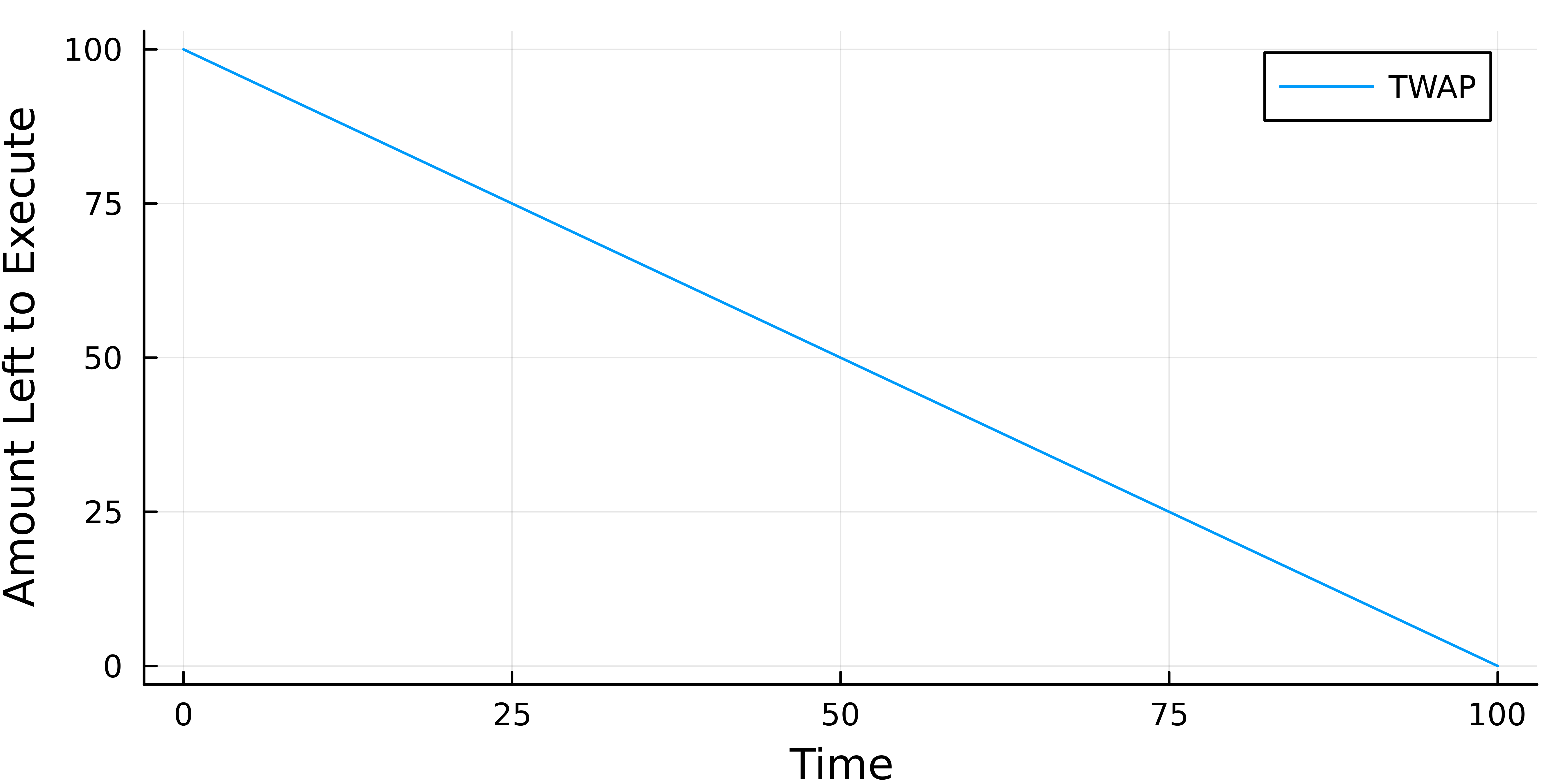
\[\int _0 ^T v_t^2\mathrm{d} t = \frac{X^2_0}{T^2} (T - 0) = \frac{X_0^2}{T}.\]When we plot this schedule we can see that the speed is constant and we are simply running a TWAP (time-weighted average price).

The maths is telling us:
- To minimise cost for an amount \(X_0\) then you should run your TWAP for an infinite amount of time.
This neglects the price risk, so sure, run a very long TWAP but don’t complain when the market trends against you!
How can we account for this price risk?
Mean-Variance Optimisation of the Almgren Chriss Model
We now need to minimise both the expected cost and the variance of the expected cost with our trading schedule. This means we will now be sensitive to cases where the price moves far away from the starting value.
We introduce a new parameter, \(\lambda\), that controls our risk aversion. So now we are worried about the price potentially running away from us if we take too long to finish the trade
\[\min _ {v_t} \left( \mathbb{E} [C] + \lambda \text{Var} [C] \right ),\]so now we want to minimise the average and the variation of the trading cost and see what schedule that produces.
When we took the expectation, only the deterministic bits remained. When we calculate the variance only the random bits remain
\[\text{Var} [C] = \mathbb{E} \left[ \sigma _0 \bar{S} _0 \int _0 ^T X_t \mathrm{d} t \right] ^2 = \sigma ^2 \bar{S}_0^2 \int _0 ^T X_t ^2 \mathrm{d} t,\]which means our minimisation problem can be written as:
\[\text{min} _{v_t} \int _0 ^T v_t ^2 \mathrm{d} t + \lambda \sigma ^2 \bar{S}_0^2 \int _0 ^T X_t ^2 \mathrm{d} t.\]Using the Euler-Lagrange equations again
\[\begin{align*} f & = A v_t^2 + B X_t^2 \\ \frac{\partial f}{\partial X} & = 2B X_t \\ \frac{\partial f}{\partial v} & = 2A v_t \\ B X_t & = A\frac{\mathrm{d} }{\mathrm{d} t} v_t \\ & = - \frac{A}{B} \frac{\mathrm{d}^2}{\mathrm{d} t^2} X_t. \end{align*}\]This is a second-order linear ordinary differential equation with solution
\[X_t = c_1 e^{\sqrt{\frac{A}{B}} t} + c_2 e ^{- \sqrt{\frac{A}{B}} t},\]Again, applying boundary conditions
\[X_0 = c_1 + c_2,\] \[X_T = 0 = c_1 e^{\sqrt{\frac{A}{B}} T} + c_2 e^{-\sqrt{\frac{A}{B}T}},\] \[X_t = X_0 \frac{\text{sinh} \sqrt{\frac{\eta}{\lambda \sigma ^2 \bar{S}_0}} T-t}{\text{sinh} \sqrt{\frac{\eta}{\lambda \sigma ^2 \bar{S}_0}} T}.\]Which is a funny expression, but underneath it is just an exponential.
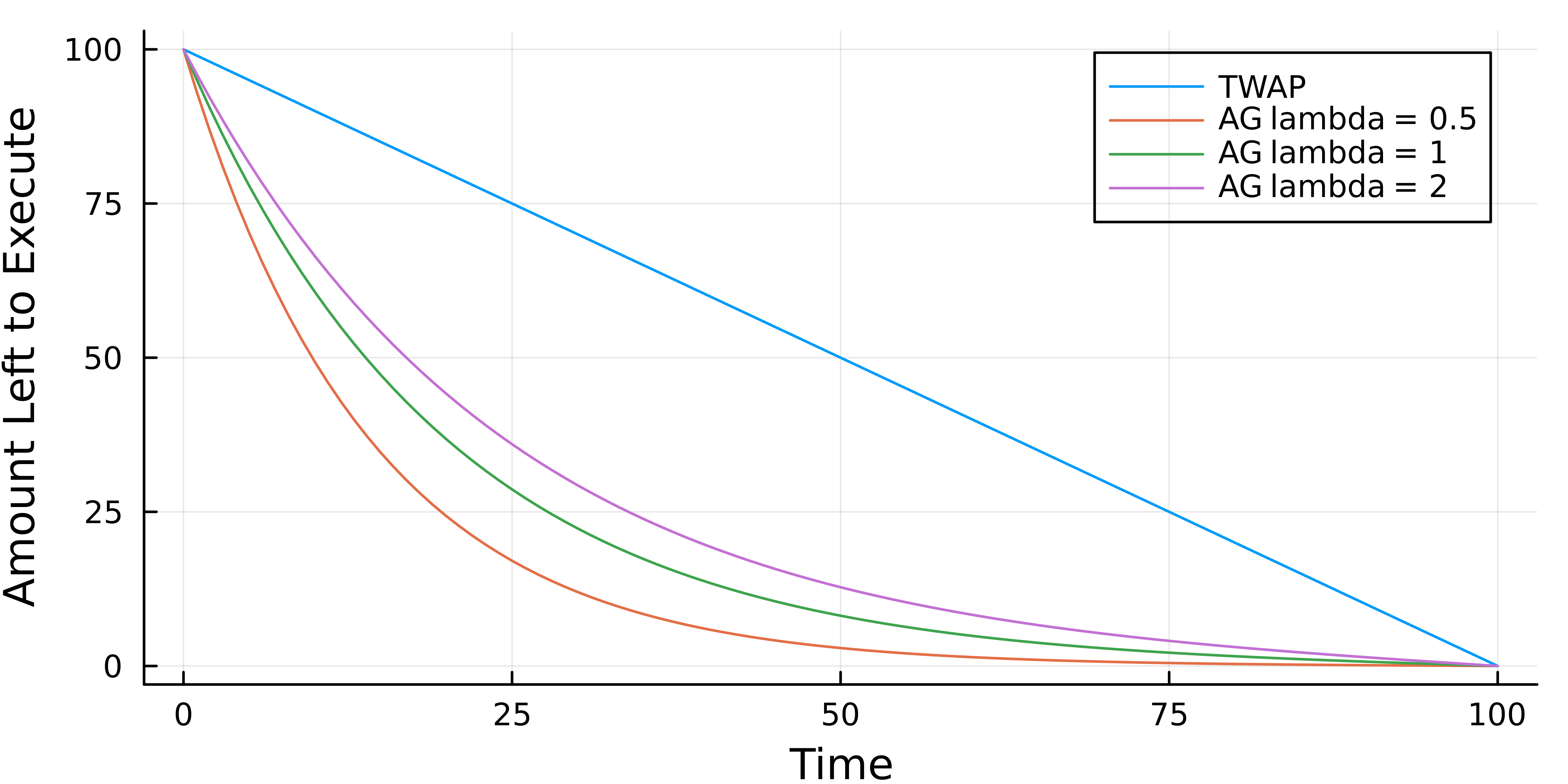
We now have the additional \(\lambda\) parameter and so plot the execution schedule for different risk aversions

A higher \(\lambda\) means a higher risk tolerance so it becomes closer to the TWAP. In general, we can see that the Almgren Chriss solution is front-loaded - most of the trading is done early on in the time window.
Summary
Ok maths over, put down your pencils and breathe. We’ve gone through the full problem set-up and show how the TWAP minimises expected costs for a risk-neutral investor and how an exponential execution schedule minimises cost for a risk-sensitive investor.
Now we know the maths we can go on to do some interesting things.