Importance Sampling, Reinforcement Learning and Getting More From The Data You Have
A new paper hit my feed Choosing trading strategies in electronic execution using importance sampling. I’ve only encountered sampling as part of a statistical computing course as part of my PhD, and I had never strayed away from Monte Carlo sampling, but this practical example provided an intuitive understanding of its importance and utility.
Enjoy these types of posts? Then you should sign up for my newsletter.
The key tenet of the paper is to use the data you have to evaluate a strategy you are considering without actually running the new strategy in production. In real life, changing something like these strategies can take a long time, with limited upside but unlimited downside if it all goes wrong.
This blog post will run through the paper and replicate the main themes in Julia. I believe the author is a Julia user too, I remember enjoying their JuliaCon talk about high-frequency covariance matrices - HighFrequencyCovariance: Estimating Covariance Matrices in Julia and the associated Julia package HighFrequencyCovariance.jl
The Execution Traders Problem
You are an execution trader with access to 4 different broker algorithms (algos) to execute your trade. With each trade you need to choose an algo and measure the trade’s overall slippage - the price you paid vs the price at the start of the order. You want to choose the best algo to ensure each of your trades gets the best price.
How do you choose what one to use? Do you have enough data to decide what one is the best one? Is any one algo better than the other? These are all difficult questions to answer but with some data on how the algos performs you should be able to use the data to help inform your decision.
We are trying to maximise the performance of each trade by choosing the correct algo. Our trade is described by a variable \(x\) and each algo performs differently depending on \(x\). The paper calls the performance ‘slippage’ but then tries to maximise the slippage which sounds weird to me - I always talk about minimising slippage! But that’s splitting hairs.
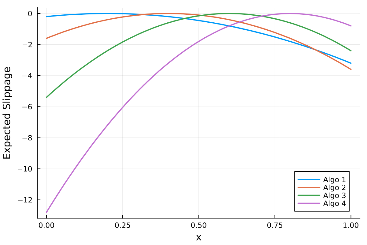
The performance of algo \(i\) is described by an analytical function with parameters \(\alpha _i, \beta _i\) plus some noise that depends on the duration of the trade \(d\) and the volatility \(\sigma\).
function expSlippage(x, alpha, beta)
   @. -alpha*(x - beta)^2
end

function slippage(x, alpha, beta, d, sigma)
    expSlippage(x, alpha, beta) + rand(Normal(0, d*sigma/2))
end
The \(\alpha\)’s and \(\beta\)’s are simple constants set in the paper.
alphas = [5,10,15,20]
betas = [0.2, 0.4, 0.6, 0.8]

x = collect(0:0.01:1)
p = plot(xlabel = "x", ylabel = "Expected Slippage")
for i in eachindex(alphas)
   plot!(p, x, expSlippage(x, alphas[i], betas[i]), label = "Algo " * string(i), lw = 2)
end
p

Here we can see where each algo is better for each \(x\). In reality, this is impossible to know or it might not even exist.
We are going to devise a rule of when we will select each trading algo:
-
If \(x<0.5\) then we will randomly select Strategy 1 62.5% of the time and the others 12.5% of the time.
-
If \(x>0.5\) then Strategy 3 62.5% and the others 12.5%.
function tradingRule(x)
    if x < 0.5
        return [0.625, 0.125, 0.125, 0.125]
    else
        return [0.125, 0.125, 0.625, 0.125]
    end
end
Julia’s vectorisation makes it easy to simulate going through multiple trades.
x = rand(Uniform(), 100)
d = rand(Uniform(), 100)
stratProbs = tradingRule.(x)
strat = rand.(Categorical.(stratProbs))
stratProb = getindex.(stratProbs, strat)
slippageVal = slippage.(x, alphas[strat], betas[strat], d, 5)

res = DataFrame(x=x, d=d, strat=strat, stratProb=stratProb, prob=stratProb, slippage=slippageVal)
first(res, 3)
| x | d | strat | stratProb | prob | slippage |
|---|---|---|---|---|---|
| 0.0192748 | 0.95432 | 1 | 0.625 | 0.625 | 1.29969 |
| 0.0700494 | 0.930581 | 1 | 0.625 | 0.625 | 0.855019 |
| 0.925858 | 0.90087 | 3 | 0.625 | 0.625 | -2.62943 |
This is our ‘production data’ for 100 random trades. The aim of the game is to understand how good our trading rules are rather than trying to estimate how good the individual algos are.
Does our rule above do better than just randomly choosing an algo? This is where we can use importance sampling to take the 100 trades and specially weight them to assess a new trading rule.
Importance Sampling
Importance sampling is about using observed probabilities \(q\) and observations of a variable with different probabilities \(p\). In our case we want to calculate the expected slippage of a trading strategy given the observations we have of the current strategy.
\[\mathbb{E} [\text{Slippage}] = \frac{1}{N} \sum _i \text{Slippage}_i \frac{p_i(\text{New Strategy})}{q_i(\text{Current Strategy})}\]\(q_i(\text{Current Strategy})\) is equal to the stratProb column in the dataframe and \(p_i\) is the probability we would have chosen the given algo under the new strategy.
For the importance sampling, we calculate the likelihood ratio using equal probabilities and then take the weighted average of the slippages.
res = @transform(res, :EqProb = 0.25)
res = @transform(res, :ratio = :EqProb ./ :stratProb)
@combine(res, :StratSlippage = mean(:slippage), :EqStratSlippage = mean(:slippage, Weights(:ratio)))
| StratSlippage | EqStratSlippage |
|---|---|
| -1.02243 | -1.8774 |
The average slippage for the 100 trades is worse (more negative) that the current strategy. This suggests that randomly choosing would perform worse.
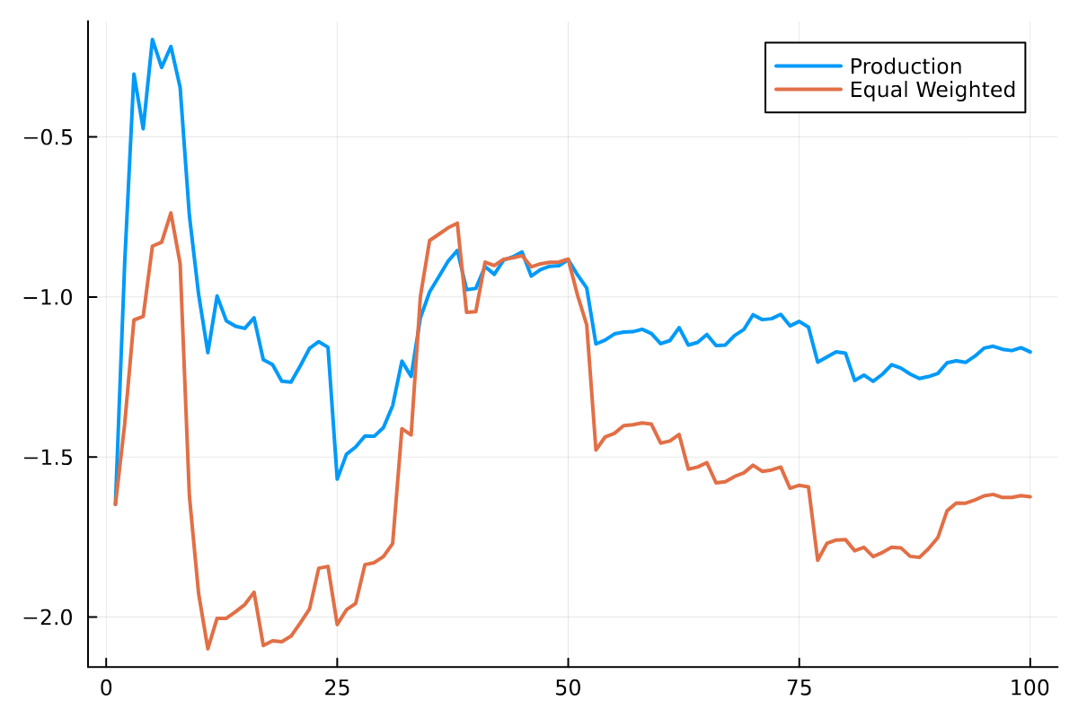
Then plotting the average slippage across the orders.
res = @transform(res, :StratSlipapgeRolling = cumsum(:slippage) ./collect(1:length(:slippage)))
res = @transform(res, :EqSlipapgeRolling = cumsum(:slippage .* :ratio) ./cumsum(:ratio))

plot(res.StratSlipapgeRolling, label = "Production", lw =2)
plot!(res.EqSlipapgeRolling, label = "Equal Weighted", lw =2)

The timeseries of the slippage shows that the equally weighted strategy is worse, so gives us confidence in the current strategy. When we observe a bad outcome the likelihood ratio weights that outcome based on how different the probability is from the production strategy.
How can we use importance sampling to build better strategies?
Easy Reinforcement Learning and Expected Slippage
Each trade is described by \(x\). In this toy model that is just a number but in real life this could correspond to the size of the order, the asset, the time of day and any combination of variables. In the original paper they use the spread, volatility, order size relative to the ADV and duration as descriptive variables of a random dataset. I’m going to keep it simple and stick to \(x\) being just a single number.
We want to understand if a particular \(x\) means we should use algo \(i\). For this, we need to build an ‘expected slippage’ model where we use the historical \(x\) values and outcomes of using algo \(i\).
For the modelling part, we will use xgboost through MLJ.jl.
using MLJ
xgboostModel = @load XGBoostRegressor pkg=XGBoost verbosity = 0
xgboostmodel = xgboostModel(eval_metric=["rmse"]);
The inputs are \(x\) and an indicator of the chosen algo.
res2 = coerce(res[:,[:x, :strat, :slippage]], :strat=>Multiclass);

y, X = unpack(res2, ==(:slippage); rng=123);

encoder = ContinuousEncoder()
encMach = machine(encoder, X) |> fit!
X_encoded = MLJ.transform(encMach, X);

xgbMachine = machine(xgboostmodel, X_encoded, y)

evaluate!(xgbMachine,
          resampling=CV(nfolds = 6, shuffle=true),
          measures=[rmse, rsq],
          verbosity=0)
The overall regression gets an \(R^2\) of 0.5 on our 100 trade dataset - a decent model.
In this new simulation, we will fit the xgboost model on the trades to build up an expected slippage model with all the data we have so far. prepareData and fitSlippage transform the data and fit the model.
We will then use this model to predict the expected slippage (predictSlippage) for each algo and use that to selected what algo to use for a given trade.
function prepareData(x, strat, slippage)
    res = coerce(DataFrame(x=x, strat=strat, slippage=slippage), :strat=>Multiclass);
    y, X = unpack(res, ==(:slippage); rng=123);
    encoder = ContinuousEncoder()
    encMach = machine(encoder, X) |> fit!
    X_encoded = MLJ.transform(encMach, X);
    return X_encoded, y
end

function fitSlippage(x, strat, slippage, xgboostmodel)
    X_encoded, y = prepareData(x, strat, slippage)
    xgbMachine = machine(xgboostmodel, X_encoded, y)

    evaluate!(xgbMachine,
          resampling=CV(nfolds = 6, shuffle=true),
          measures=[rmse, rsq],
          verbosity=0)
    return (xgbMachine, encMach)
end

function predictSlippage(x, xgbMachine, encMachine)
    X_pred = DataFrame(x=x, strat = [1,2,3,4], slippage = NaN)
    X_pred = coerce(X_pred[:,[:x, :strat, :slippage]], :strat=>Multiclass)
    X_pred = MLJ.transform(encMach, X_pred)
    preds = MLJ.predict(xgbMachine, X_pred)
    return(preds)
end

function slippageToProb(preds)
    scores = exp.(preds) ./ sum(exp.(preds))
    p = ((0.9 .* scores) .+ 0.025) ./ sum((0.9 .* scores) .+ 0.025)
    return p
end
The predicted slippage is then transformed into a probability using the softmax function (slippageToProb) which gives us a mapping of the real-valued estimated slippage onto a probability. We then sample which strategy to use from this probability. By adding an element of randomness into the algo selection we are making sure we can use the importance sampling framework to either change the model (xgboost to something else) or change how we build the probabilities (softmax to something else).
To simulate the problem we will start by randomly choosing a strategy for the first 200 runs. After this we will start using the xgboost regression model to predict the expected slippage of each strategy and use this to decide what strategy to use.
epsilon = 0.05
volatility = 5
N = 1000

x = zeros(N)
strat = zeros(N)
slippages = zeros(N)
d = zeros(N)
stratProb = zeros(N)

for i in 1:N
    xVal = rand(Uniform())
    dVal = rand(Uniform())

    if i > 200
        xgbMachine, encMachine = fitSlippage(x[1:i], strat[1:i], slippages[1:i], xgboostmodel)
        predCost = predictSlippage(xVal, xgbMachine, encMachine)
        stratProbs = slippageToProb(predCost)
    else
        stratProbs = [0.25, 0.25, 0.25, 0.25]
    end

    stratVal = rand(Categorical(stratProbs))
    slippageVal = slippage(xVal, alphas[stratVal], betas[stratVal], dVal, volatility)

    x[i] = xVal
    strat[i] = stratVal
    stratProb[i] = stratProbs[stratVal]
    slippages[i] = slippageVal
    d[i] = dVal
end

res = DataFrame(x=x, d=d, strat=strat, stratProb=stratProb, slippage=slippages)
Again, we output each strategy and the probability the strategy was used. We use the importance sampling approach to estimate the slippage for choosing an algo randomly to gives us a comparison to the xgboost method.
res = @transform(res, :EqProb = 0.25)
res = @transform(res, :EqRatio = :EqProb ./ :stratProb)
res = @transform(res, :StratSlipapgeRolling = cumsum(:slippage) ./collect(1:length(:slippage)))
res = @transform(res, :EqSlipapgeRolling = cumsum(:slippage .* :EqRatio) ./cumsum(:EqRatio));

plot(res.StratSlipapgeRolling[50:end], label = "Production")
plot!(res.EqSlipapgeRolling[50:end], label = "Equal Weighting")

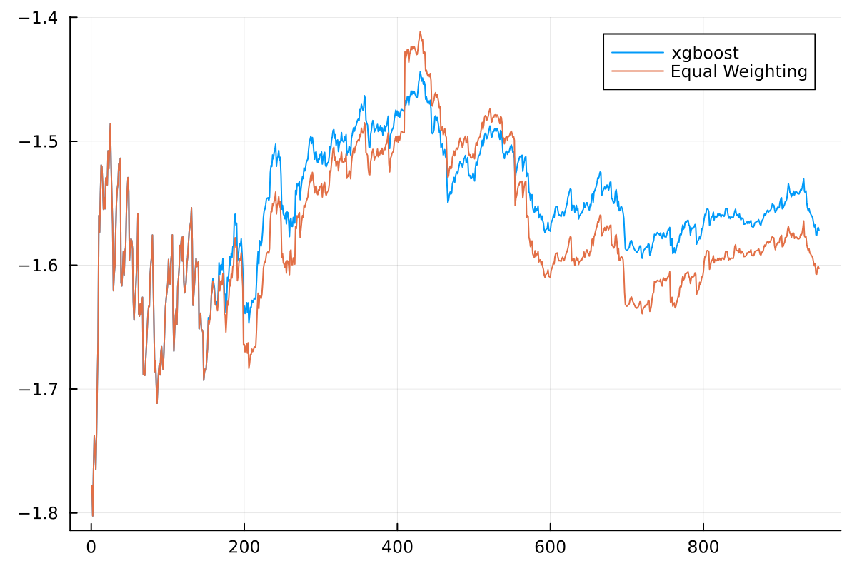
For the first 200 trades we are just selecting randomly, so no difference in performance. Then afterwards we can see the XGBoost model starts to outperform as it learns what algo is better for each \(x\). So whilst we have only run the XGBoost model in production it has shown it is doing better than random by using the importance sampling method.
Testing a New Model Without Running it in Production
The XGBoost model is doing well and out-performing an equal weighted model, but what if you wanted to change from XGBoost to something else? How can you build the case that this is something worth doing?
By constructing new probabilities of whether the strategy would be selected (new \(p_i\)’s) and with the current strategy probabilities (\(q_i\)’s) we can estimate the slippage of the new model without having to run any more trades.
With MLJ.jl we can create a new model and pass it into the functions to replicate running the strategy in production. This time we use a simple linear regression model with the same features. We run through the trades in the same order so there is no information leakage.
@load LinearRegressor pkg=MLJLinearModels

linreg = MLJLinearModels.LinearRegressor()

newProb = ones(N) * 0.25

for i in 1:(N-1)

    if i > 200
        linMachine, enchMachine = fitSlippage(res.x[1:i], res.strat[1:i], res.slippage[1:i], linreg)
        predSlippage = predictSlippage(res.x[i+1], linMachine, enchMachine)
        stratProbs = slippageToProb(predSlippage)
        newProbVal = stratProbs[Int(res.strat[i+1])]
        newProb[i] = newProbVal
    end

end

res[:, :LinearProb] = newProb

res = @transform(res, :LinearRatio = :LinearProb ./ :stratProb)
res = @transform(res, :LinearSlipapgeRolling = cumsum(:slippage .* :LinearRatio) ./cumsum(:LinearRatio))
plot(res.StratSlipapgeRolling[50:end], label = "Production")
plot!(res.EqSlipapgeRolling[50:end], label = "Equal Weighting")
plot!(res.LinearSlipapgeRolling[50:end], label = "Linear Model")

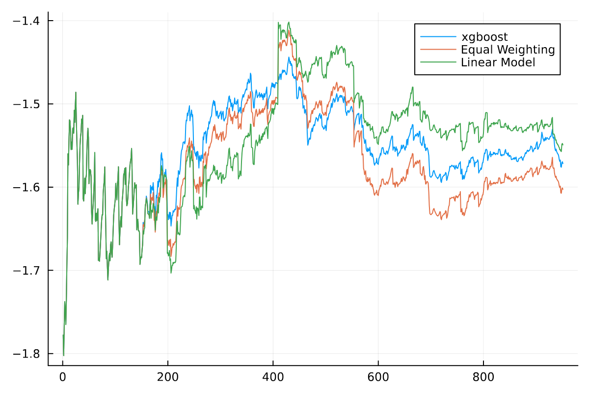
Adding the linear regression decision rule to the data gives us a way of assessing this new model without having to run it directly in production. We can see that the linear model is better than XGBoost and also better than the equal weighting.
A simple bootstrap of taking the average slippage for each strategy a random amount of times provides the simplest performance measure.
bs = mapreduce(x-> @combine(res[sample(201:nrow(res), nrow(res)-200), :],
              :StratSlippage = mean(:slippage),
              :EqStratSlippage = mean(:slippage, Weights(:EqRatio)),
              :LinearStratSlippage = mean(:slippage, Weights(:LinearRatio))),
			  vcat, 1:1000);

@combine(groupby(stack(bs), :variable), :avg = mean(:value), :sd = std(:value))
| variable | avg | sd |
|---|---|---|
| StratSlippage | -1.55385 | 0.0967389 |
| EqStratSlippage | -1.59169 | 0.119028 |
| LinearStratSlippage | -1.52706 | 0.133231 |
As it’s a toy problem, nothing of significance between the models - but both models do better than the random allocation.
Conclusion
Importance sampling gives you a way of getting more out of the current data and strategy you are using. By weighting the observations in a new way you can get an idea whether a new strategy is worth it or not. By rethinking your current setup you can easily add a bit of randomness into decisions and use the importance sampling framework going forward.