Cyclical Embedding
Cyclical embedding (or encoding) is a basic transformation for numerical variables that follow a cycle. Let’s explore how they work.
I am currently attending a Deep Learning in Finance lecture series (lectured by Stefan Zohran in preparation for his new book). The ongoing homework is taking a basic time series model and applying the various deep learning techniques. In the process of doing this homework, I’ve come across Cyclical Embeddings and how they are used to transform variables that move into a cycle into something a model can understand.
Consider this blog post me reading this Kaggle notebook: Encoding Cyclical Features for Deep Learning, converting it to Julia and using some examples to convince myself Cyclical Embeddings work and are useful.
Enjoy these types of posts? Then sign up for my newsletter.
Cyclical variables are especially pertinent in Finance. For example, day of the week you could either use a factor (the label directly) or number (Mon=1, Tue=2 etc.) in a model. Using a factor, your model now includes 5 additional parameters. If you use the number you’ll have to specify the form of the relationship (linear or using a GAM). Each has its ups and downs, but there is also a key piece of information missing: the days of the week form a cycle where 1 follows from 5. How can we translate this into something the model will understand?
As the name suggests, cyclical embeddings lead to a cycle and the natural functions are the trigonometry sin and cos. We take the one-dimensional variable and transform it into two dimensions
\[\begin{align*} x & = \sin \left( \frac{2 \pi t}{\text{max} (t)} \right), \\ y & = \cos \left( \frac{2 \pi t}{\text{max} (t)} \right). \end{align*}\]If we apply this transformation to our day of the week we go from \(t \in [0, 4]\) to a circle in \(x\) and \(y\).
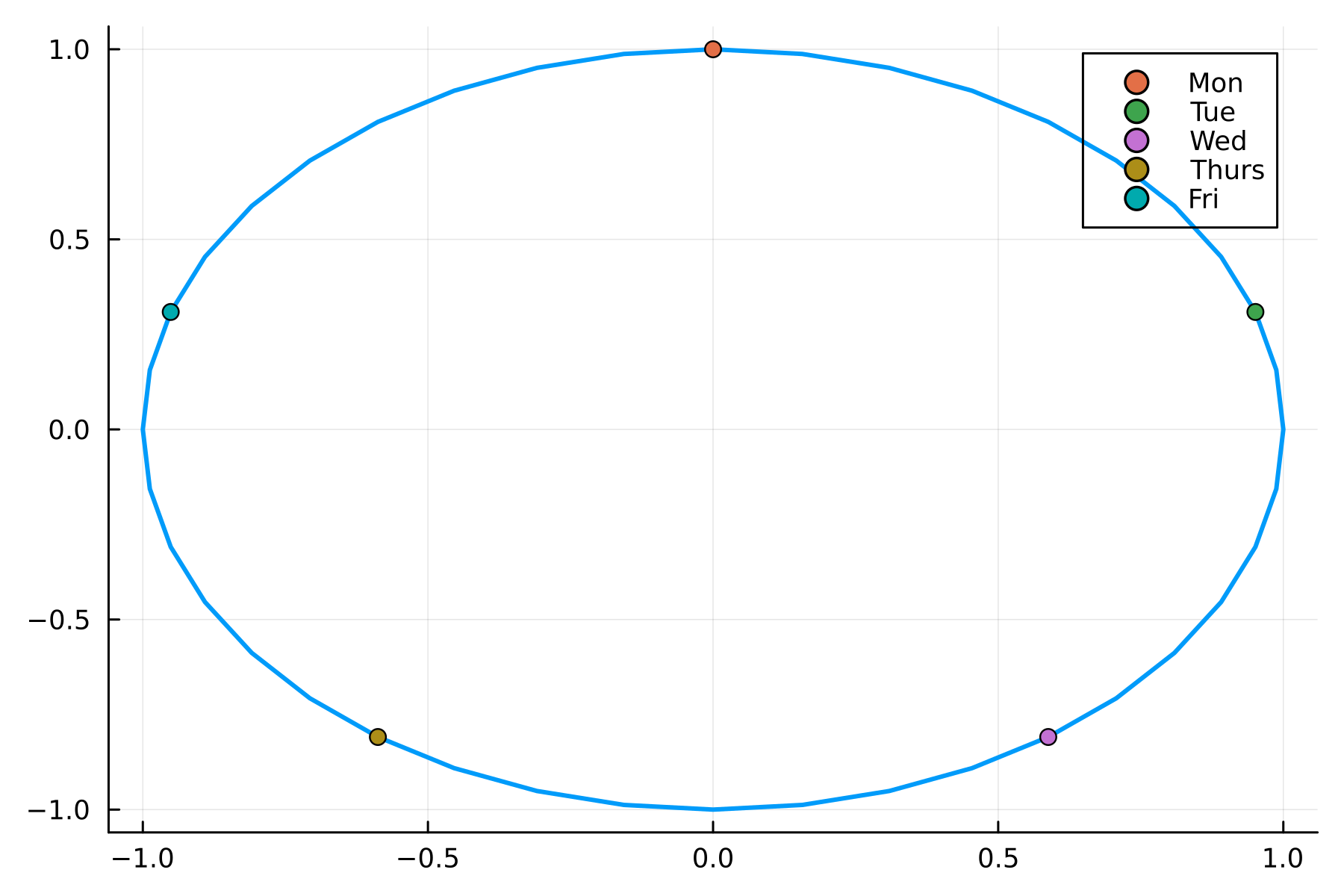
I am reminded of polar coordinates and we can now see that Monday is the same distance from Friday as it is Tuesday. Crucially, the new variables are nicely bounded between -1 and 1 which is always helpful when building models. All in, this looks like a sensible transformation, now to see if it has a noticeable difference in modelling performance.
Practical Cyclical Embeddings - Daily Volumes
Let’s model the daily trading volume of a stock. It feels logical that the day of the week (Mon-Fri), day of the month (1-31) and month (1-12) would affect the amount traded. The summer months might be quieter, the end of the month might be busier (month-end rebalancing) and Fridays might be quieter. All three of these time variables are cyclical so the cyclical embeddings should help.
We have 3 separate choices:
- Everything as a number (3 free parameters)
- Days of the week and months as factors (5 + 12 + 1 free parameters)
- Cyclically embedded the three variables (3x2=6 parameters)
So a balance between the number of parameters and the flexibility of the model.
We will use a simple linear model, nothing fancy.
As always we will be in Julia.
using Dates, AlpacaMarkets, Plots, StatsBase, GLM
using DataFramesMeta, CategoricalArrays, ShiftedArrays
To load the data in we will use my AlpacaMarkets.jl API and pull in as much daily data as possible.
aaplRaw, npt = AlpacaMarkets.stock_bars("AAPL", "1Day"; startTime=Date("2000-01-01"), endTime = today() - Day(2), adjustment = "all", limit = 10000)
Some basic cleaning and formatting.
aapl = aaplRaw[:, [:t, :v]]
aapl[!, "t"] = DateTime.(chop.(aapl[!, "t"]))
Julia makes it easy to add the factor variables and the numeric versions. As the numeric values all start at 1 we subtract one so they begin at 0.
aapl[:, :DayName] = CategoricalArray(dayname.(aapl.t))
aapl[:, :MonthName] = CategoricalArray(monthname.(aapl.t))

aapl[:, :DayOfMonth] = dayofmonth.(aapl.t) .- 1
aapl[:, :DayOfWeek] = dayofweek.(aapl.t) .- 1
aapl[:, :MonthOfYear] = month.(aapl.t) .- 1;
We normalise the volume to millions of shares and take the difference.
aapl = aaplRaw[:, [:t, :v]]
aapl[:, :vNorm] = aapl[:, :v] .* 1e-6;
aapl[:, :delta_vNorm] = aapl[:, :vNorm] .- ShiftedArrays.lag(aapl[:, :vNorm]);
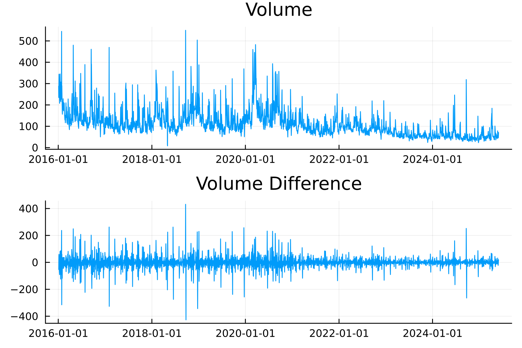
As the regular volumes (vNorm) aren’t stationary, we can see a clear trend that changes, it’s better to model the difference in volumes each day.
plot(plot(aapl.t, aapl.vNorm, title = "Volume", label = :none),
     plot(aapl.t, aapl.delta_vNorm, title = "Volume Difference", label = :none), layout=(2,1))
To apply the cyclical encoding we need to take one column and turn it into two.
function cyclical_encode(df, col, max)
    df[:, Symbol("$(col)_sin")] = sin.(2 .* pi .* df[:, Symbol(col)]/max)
    df[:, Symbol("$(col)_cos")] = cos.(2 .* pi .* df[:, Symbol(col)]/max)
    df
end

for col in ["DayOfWeek", "DayOfMonth", "MonthOfYear"]
    aapl = cyclical_encode(aapl, col, maximum(aapl[:, col]))
end
If you’ve not seen it before the $ is like Python F-strings and lets you use a variable in the string.
We do the normal test/train split.
aaplTrain = aapl[1:2000,:]
aaplTest = aapl[2001:end,:];
Now to build the three models.
The numerical model takes in the numbers directly.
numModel = lm(@formula(delta_vNorm ~ DayOfWeek + MonthOfYear + DayOfMonth), aaplTrain)
The factor model represents the day of the week and day of the month as categories so they each get a separate parameter.
factorModel = lm(@formula(delta_vNorm ~ DayName + MonthName + DayOfMonth + 0), aaplTrain)
The embedding model takes in the sin/cos transformation of each of the variables.
embeddingModel = lm(@formula(delta_vNorm ~ DayOfWeek_sin + DayOfWeek_cos + DayOfMonth_sin + DayOfMonth_cos + MonthOfYear_sin + MonthOfYear_cos), aaplTrain);
To assess how well the models perform we look at the RMSE (in sample and out of sample), AIC (in sample) and \(R^2\) (in sample and out of sample).
| Model | NumCoefs | RMSE | RMSEOOS | AIC | R2 | R2OOS |
|---|---|---|---|---|---|---|
| Numeric | 4 | 31.1041 | 50.2975 | 21346.9 | 0.0336539 | 0.0396665 |
| Factor | 17 | 31.2978 | 50.0453 | 21352.8 | 0.0433269 | 0.0276647 |
| Embedding | 7 | 31.7484 | 51.1591 | 21420.8 | 0.0002655 | -0.000531 |
Interestingly, the embedding model performs the worst both in sample and out of sample.
When we pull out the Day of the Week effect it’s easy to see what the model has learnt.
params = Dict(zip(coefnames(embedingExample), coef(embedingExample)))

x = 0:0.1:4
ySin = params["DayOfWeek_sin"] * sin.(2 .* pi .* x ./ maximum(x))
yCos = params["DayOfWeek_cos"] * cos.(2 .* pi .* x ./ maximum(x))


p = plot(x, ySin, label = "Sin")
plot!(p, x, yCos, label = "Cos")
plot!(p, x, yCos .+ ySin, label = "Combined")
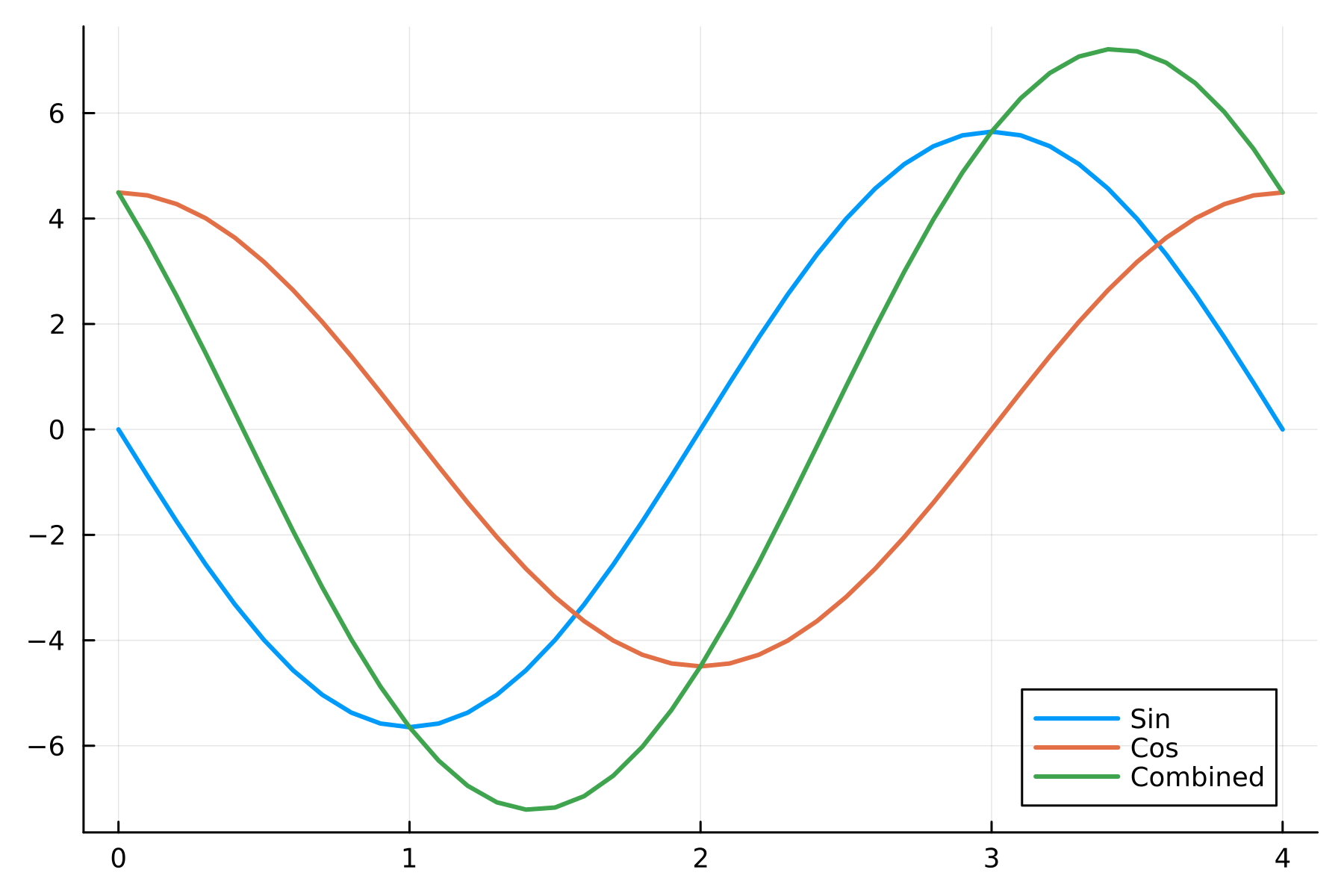
This indicates the lower volume changes are on Tuesday and the higher volume changes are on Thursday.
Based on the model performance it’s not a great showing for the embedding transformation. Let’s move on to another example where the cyclical nature might be more obvious.
Practical Cyclical Embeddings - Intraday Volumes
Another example would be the flow of trades over the day. In this case, the hour is the variable we will cyclically embed. For this, we use BTCUSD trades from AlpacaMarkets.jl and aggregate them over the day.
btcRaw, token = AlpacaMarkets.crypto_bars("BTC/USD", "1H"; startTime=Date("2025-01-01"), limit = 10000)

res = [btcRaw]
while !(isnothing(token) || isempty(token))
    println(token)
    newtrades, token = AlpacaMarkets.crypto_bars("BTC/USD", "1H"; startTime=Date("2025-01-01"), limit = 10000, page_token = token)
    println((minimum(newtrades.t), maximum(newtrades.t)))
    append!(res, [newtrades])
    sleep(AlpacaMarkets.SLEEP_TIME[])
end
res = vcat(res...);
Sidenote, I do need to wrap this functionality into the package itself.
We get the raw data into a suitable state.
btc = res[:, [:t, :v]]
btc[!, "t"] = DateTime.(chop.(btc[!, "t"]));

btc = @transform(btc, :Date = Date.(:t), :Time = Time.(:t), :DayOfWeek = dayofweek.(:t), :Hour = hour.(:t))
trainDates = unique(btc.Date)[1:140]
testDates = setdiff(unique(btc.Date), trainDates)

trainDataRaw = btc[findall(in(trainDates), btc.Date), :];
testDataRaw = btc[findall(in(testDates), btc.Date), :];

trainData = @combine(groupby(trainDataRaw, [:Hour]), :v = sum(:v))
trainData = @transform(trainData, :total_v = sum(:v), :frac = :v./sum(:v))

testData = @combine(groupby(testDataRaw, [:Hour]), :v = sum(:v))
testData = @transform(testData, :total_v = sum(:v), :frac = :v./sum(:v))

sort!(trainData, :Hour);
sort!(testData, :Hour);
Again, using a linear model we fit the embedded hour variables to the fraction of the volume traded per hour.
embedModelIntra = lm(@formula(frac ~ Hour_sin + Hour_cos), trainData)
When comparing the results, we are now just looking at the intraday profile of the trades for both the train set and test set overlaid with the model.
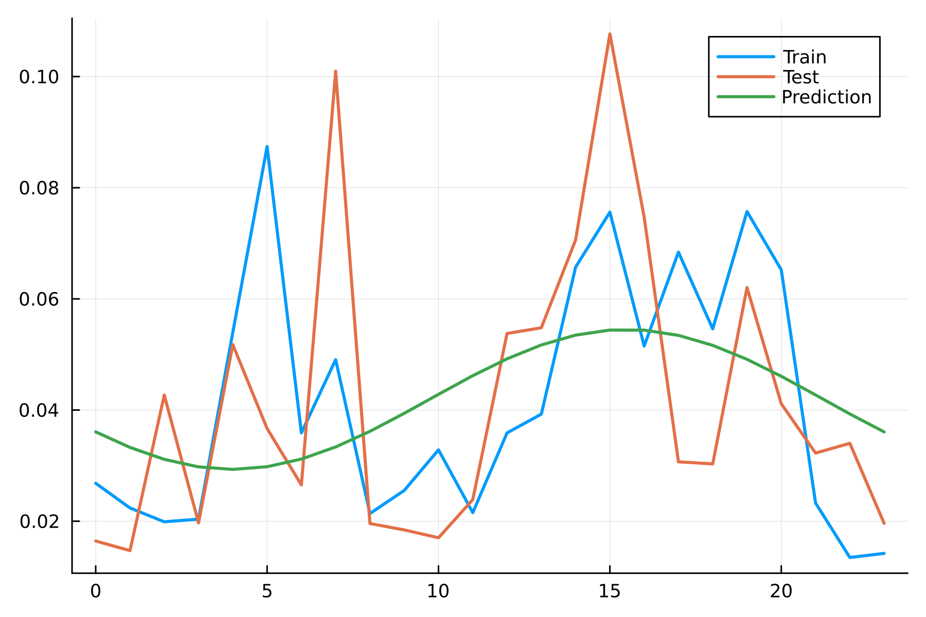
The model has done well to pick up the peak in the afternoon but has missed the peak in the early morning. The RMSE of this model is 0.029 vs 0.026 from using the training fractions directly, so again the encoded model has done worse. This is the limiting factor with this embedding, we have a single frequency of sin/cos when in reality this problem needs more degrees of freedom, i.e. multiple components
\[\sum _i c^1_i \sin \left(\frac{2 \pi \omega _i x}{\max (x)}\right) + c^2_i \cos \left(\frac{2 \pi \omega _i x}{\max (x)}\right).\]This is now a GAM with trigonometric splines so we can view the cyclical encoding as a 1-spline GAM.
Conclusion
It’s an interesting transformation of time-like variables and gives you a route to smoothing out the beginning and ending of the cycles.
In these toy models, the embedding hasn’t improved performance but it’s possible that it’s more relevant in deep learning architectures where there are more parameters and more interactions. In all the above models there’s much more groundwork to do before we start eeking out performance gains from the time variables.