Point Process Estimation with dirichletprocess
My R package dirichletprocess can easily estimate the intensity
function of a point process. I use a Bayesian
nonparametric method to infer the intensity function as a mixed
model.
require(dplyr)
require(tidyr)
require(ggplot2)
require(dirichletprocess)
require(boot)
In my first tutorial, Density Estimation with the dirichletprocesss R package I demonstrated how you can use the dirichletprocess package to estimate densities using nonparametric Bayesian mixtures. In the second tutorial I showed how easy it is to add in your own conjugate mixture models. In part three of this tutorial series I will show how you can use a Dirichlet process to estimate a point process model.
But firstly what is a point process? Wikipedia states that a point process is a collection of points randomly located on some space. So, if we have a rectangle, a collection of random points inside the rectangle is a point process. For example, lets say we have a field where flowers are growing randomly. The co-ordinates where each flower is located form a point process. Or, in a 1 dimensional example, we might be observing how long it takes for a bus to arrive at a bus stop. Each time a bus arrives, the time is noted. These collection of bus arrival times form a 1D point process.
Point processes appear all the time in finance. Last month I wrote about extreme values in the VIX index. Every time the VIX breaks a set threshold can be thought of as a point process. Or even every time a stock is traded is a point process.
In this example we will be looking at coal mining disasters using the
coal dataset from the boot package. This is a classic point
process example that records the dates of coal mine explosions that resulted in 10 or more deaths.
qplot(coal[,1], geom="histogram", binwidth=1, )

Here we can see that the rate of accidents is not constant. There was quite an increase in accidents from 1850 til 1875 when the number of accidents declined. At the turn of the 20th Century, accidents were fairly constant until 1925 when they started increasing. This type of non-constant pattern suggests an inhomogeneous Poisson process might be an improvement on a basic Poisson process.
An Inhomogeneous Point Process Model
We think that the event times are distributed from an inhomogeneous Poisson process with rate \(λ(t)\). We will decompose this rate into two components, a amplitude \(λ_0\) and a density \(f(t)\). We will use a Dirichlet mixture of Beta distributions to model \(f(t)\). The amplitude \(λ_0\) will be estimated using conjugate Gamma prior distribution to draw from the prior.
As the Beta mixture is a default model from the dirichletprocess
package, we can easily construct fit our density part of the
model. The data window is from 15/03/1851 to 22/03/1962, therefore we
must subtract this start time from each observation to arrive at
\(t_i\)’s in \(\left[0, T \right]\).
maxT <- 1963-1851
eventTimes <- coal[,1] - 1851
dp <- DirichletProcessBeta(eventTimes, maxT, mhStep = c(0.5, 0.5))
## Accept Ratio: 0.215
dp <- Fit(dp, 500, progressBar = FALSE)
As we are fitting a nonconjugate model, we are provided with an initial acceptance ratio for the Metropolis-Hastings step in updating the parameters.
plot(dp)
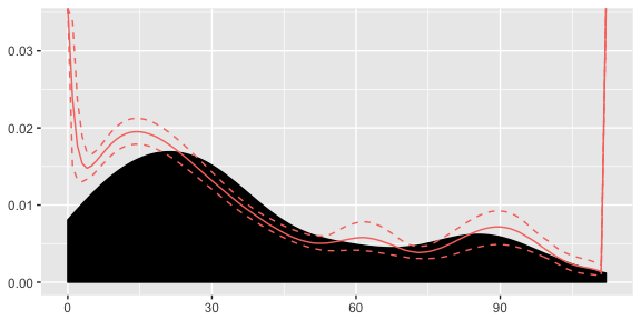
Here we can see that our density has picked up both the peaks in the data successfully. Slight issues at the boundaries, but this is an artefact of the Beta distribution. For now we won’t be worrying about these edge effects.
Now for the amplitude part. As the prior is conjugate we can easily draw from the analytical posterior distribution. These samples are also used for a constant Poisson model.
lambda0Draws <- rgamma(100, length(eventTimes)+0.01, 1 + 0.01)
For the constant Poisson point process our density \(f(t)\) is simply \(\frac{1}{T}\). I.e the pdf of a uniform distribution. Out \(\lambda _0\) is the same.
Point Process Residuals
Now that we have two models, we wish to see if our more complicated inhomogeneous model is better than a constant point process model. The residuals for a point process are defined as \[ \Lambda _k = \int _ {t _k} ^{t _ {k + 1}} \lambda (t) \mathrm{d} t . \]
We can use them to compare our models. Using the time-rescaling theory, these residuals should be distributed as Poisson process with rate 1 if our \(\lambda (t)\) is the true intensity function of the process. Therefore if we calculate the residuals for both our models we can see what set of residuals are closer to the believed true residuals.
Calculating the residuals for a constant model is simple, it is just the sampled amplitude multiplied by the event differences.
residConst <- lapply(lambda0Draws, function(x) diff(eventTimes)*(x/maxT))
For the inhomogeneous model, it is slightly more involved. We must integrate our density function \(f(t)\) for each inter-event time. But by nesting a sapply inside an lapply we can calculate a set of residuals for each posterior sample. Using the PosteriorFunction function on the fitted dp object allows us to easily sample from the posterior distribution of the Dirichlet process.
residInhomo <- lapply(lambda0Draws, function(y) sapply(seq_along(eventTimes)[-length(eventTimes)], function(i) integrate(PosteriorFunction(dp), lower=eventTimes[i], upper=eventTimes[i+1])$value * y))
Using residual theory, we know that the residuals are distributed as a Poisson process with rate 1. That means that mean and variance of the residuals are also 1. As we have calculated the residuals for each posterior simulation we can then calculate a distribution of the mean and variance for each model. As we know that these should be 1 this allows us to arrive at a posterior p-value.
inhomoResidRes <- data.frame(Mean=sapply(residInhomo, mean),
                             Var=sapply(residInhomo, var),
                             Model="Dirichlet")
constResidRes <- data.frame(Mean=sapply(residConst, mean),
                             Var=sapply(residConst, var),
                             Model="Constant")
residRes <- bind_rows(inhomoResidRes, constResidRes)

residRes %>% gather(Parameter, Value, -Model) -> residResTidy

ggplot(residResTidy, aes(x=Value, fill=Model, colour=Model)) + geom_density() + facet_wrap(~Parameter) + geom_vline(xintercept = 1)
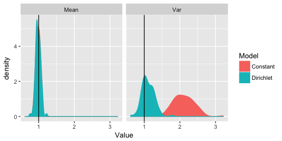
Our graph above shows that the means are suitably distributed around 1 but for the variances we can see that the constant Poisson process model is centred around 2, therefore we should reject this model as inadequate. Our inhomogeneous Beta mixture model is better suited to the data.
However, whilst this model is a better fit for explaining the trend in mining disasters, it fails in prediction. As we have chosen a fixed window over which our Beta distribution mixture is defined, anything outside that window, i.e. accidents after 1963, cannot be predicted. Our Beta mixture model does not extend into the future. Therefore we must be clear with the scope of our model.
Overall, we have introduced how a point process can be used to model specific types of data. Then using the dirichletprocess package we can build our model using a mixture of Beta distributions. We then asses the model fit using residuals and find that our inhomogeneous Poisson process is better than a standard homogeneous Poisson process before finally highlighting that our model works well for explaining, but will break down in prediction.