Clustering with Dirichlet Processes
This post is another tutorial on using my dirichetprocess package in R. So far I have shown you how to perform density estimation, point process inference, and adding your own custom mixture model. In this tutorial I will show you how Dirichlet processes can be used for clustering.
Before we being, make sure you download the latest version of the package from CRAN.
install.packages("dirichletprocess")
We then load a few helper packages
library(ggplot2)
library(dirichletprocess)
library(dplyr)
For our data we will be using the classic faithful dataset, as we did in the density estimation. But this time we will use both columns of the data.
First lets take a look at the data.
ggplot(faithful, aes(x=waiting, y=eruptions)) + geom_point()
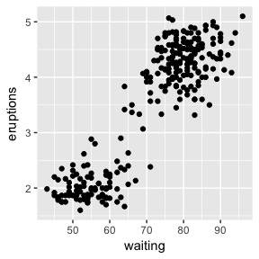
There is a clear split and two distinct clusters of the data. The length of waiting time between eruptions is positively correlated with the length of that eruption. Those with a waiting time of more than 70 minutes have eruptions lasting more than 3 minutes most of the time.
With a Dirichlet process we can perform some unsupervised machine learning and group the data based on common clusters. Mathematically, we think that the pair of observations are drawn from a multivariate normal mixture distribution.
\[(\text{waiting}, \text{eruptions})_i \sim N(\mu _i, \sigma _i)\]where \(\mu\) is a 2 dimensional vector of the mean, \(\sigma\) is the covariance matrix and \(i\) labels the cluster parameter.
We think that these parameters are drawn from a Dirichlet process
\[\mu _i , \Sigma _i \sim \text{DP} (\alpha, G_0)\]. Where \(\alpha\) is the concentration of the Dirichlet process and \(G_0\) is the base measure. This is a conjugate problem, so \(G_0\) is just the conjugate prior for a multivariate normal model.
But as you are using a the dirichletprocess package, you don’t have
to worry about any of this maths. You can simply build a
dirichletprocess object and pass the data in to find the appropriate
clusters. Again, remember to scale your data, the priors for this model
are defined such that the data is distributed around 0.
faithfulTrans <- scale(faithful)

dp <- DirichletProcessMvnormal(as.matrix(faithfulTrans))
dp <- Fit(dp, 1000, progressBar=FALSE)
plot(dp)
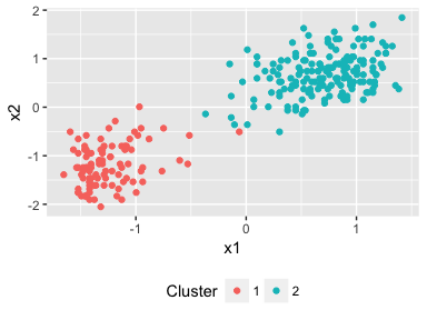
Two clusters have been found by the Dirichlet process and where we would expect to see them aswell. Out of the box we can perform unsupervised clustering in just 3 lines of code!
What if we have more than two dimensions, how does that change things? Thankfully it doesn’t and the procedure remains the same. You can still easily fit using the same functions - just passing in your data matrix.
Again, using classic stats data sets we can perform some basic
clustering on the iris dataset. We use the four quantitate values of
the dataset; the lengths and widths of the sepals and petals.
iris %>% select(-Species) %>% scale -> irisPred
dp <- DirichletProcessMvnormal(irisPred)
dp <- Fit(dp, 5000, progressBar = FALSE)
pairs(irisPred, col=dp$clusterLabels)
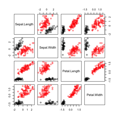
Here we show how the iris data set can be clustered into two
different groups. We’ve used the base R graphics to produce a pairs
plot with the two different clusters separated by colours. The four
dimensional set has been clustered and resulted in two different
groups. No changes needed in our Dirichlet process code.
Overall, using the Dirichlet process package you can easily perform
some unsupervised clustering. The dimensionality of your data is no
problem, at least for the software! So download dirichletprocess and
get clustering!