Fixture Difficulty and Fantasy Premier League Point Predictions
In my last blog post I showed how the odds can be used to measure the difficulty of a football match. I then took this difficulty and investigated how predictive it was for the outcome of the match (not very predictive) and the goals/shots taken in the match (more predictive).
I’m now applying the same though process to the Fantasy Premier League competition. This difficulty measure gives us a good indication of how our fantasy team should be shaped, you should prefer players that have easier matches coming, as those matches are likely to lead to more goals. Likewise, avoid defenders in these difficult matches as they are much more likely to concede and lose those clean sheet points!
Enjoy these types of posts? Then sign up for my newsletter.
The Fantasy Premier League (FPL to be short)
The whole reason and/or inspiration behind this analysis comes from wanting to be better at Fantasy Premier League. For those that don’t know this is an online game where you build a team of 11 premier league players. There is a budget and some rules on selection, but in short its about picking good players. Then, each week players score points and your total score is the sum of all your players points. I am taking the moneyball approach with my FPL team selection and trying to build models to help select my team. This will hopefully prove the superiority of a numbers based approach compared the proper footballing man methods of choosing people with ‘passion’. So far I’m 12th (out of 16) so not doing the analytics any good.
There is a whole community of people that take a stats based approach and people have even written their Master’s thesis on such topics! So my contribution to this community is a better method of assessing fixture difficulty. You can read my previous blog post on how to construct this difficulty measure but in this post I will be seeing if we can build a model that incorporates this fixture difficulty into a players predicted points for each weak. An expected points model to be concise.
This will be a simple model that is just relating the difficulty of a match to the total points scored by each player. I’ll be assuming the points are distributed Poisson like and using both xgboost for pure predictive performance and a GAM to try and understand the relationship between difficulty and total points scored.
I’ve download the data from https://github.com/vaastav/Fantasy-Premier-League which provides how many points each player achieved each week over the last few seasons. I join it with the odds data from football-data.co.uk and that gives us our full data set.
I do the usual 70/30 split randonly. I’m not worried about using future games to predict previous, more about just understanding the underlying structure in how points are scored.
require(caret)

fplModelData <- read_csv("data/player_clean_data.csv") %>%
  drop_na(Difficulty, position) %>%
  mutate(position = factor(position, levels = c("GK", "DEF", "MID", "FWD")),
         total_points =if_else(total_points < 0, 0, total_points))

trainIndexes <- createDataPartition(fplModelData$total_points, p = 0.7, list=F)

fplModelData[trainIndexes, ] -> trainData
fplModelData[-trainIndexes, ] -> testData
It is a simple model, I am just including the fixture difficulty, the value of the player and what position they play in and all second order effects. The difficulty will be a non-linear spline for each position category.
gamModel <- gam(total_points ~ s(Difficulty, by=position) + (value + position)^2,
                  data=trainData,
                  family="poisson",
                  method="REML")
This fits pretty quickly so we can move onto understanding how difficulty effects the total points for each position.
ggplot(pltFrame, aes(x=Difficulty,
                                 y=exp(Fit),
								 ymin=exp(Fit - 1.96*SE),
								 ymax = exp(Fit + 1.96*SE),
								 colour=as.factor(Position),
								 fill=as.factor(Position))) +
  geom_line() +
  geom_ribbon(alpha=0.5) +
  facet_wrap(~Position, scales="free_y") +
  theme(legend.position = "none", legend.title = element_blank()) +
  ylab("Expected Points Effect") +
  scale_color_brewer(palette = "Dark2") +
  scale_fill_brewer(palette="Dark2")
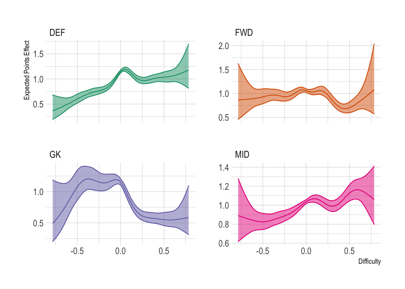
Couple of interesting things to note here.
- Goalkeepers actually score more points in difficulty matches.
This is because they get points for making more saves and this is more likely to happen in the difficult matches where they are facing more shots. You probably don’t want to be switching goals keepers when they have difficult matches though, as its probably more likely they will also lose their clean sheet bonus, which is enough to wipe out the extra points from a few extra saves.
- Defenders and midfielders have a linear increase in points worth about 1 point from difficult to easy matches.
What is interesting though is the relative flatness of the forwards plus the slight decrease in matches with a difficulty around 0.25 to 0.5 before the quick increase in very easy matches.
XGBoosting
Now we know there is a link between difficulty and expected points, what if we just throw interpretability to the wind and build the most predictive model possible? For this I will use a tree based model implemented with the xgboost library. I’ll include all the same variables as above and up to second order interactions. Let’s see if we can improve the GAM.
This model can take a while to fit (about 20 minutes) so I take advantage of multiple cores and adaptive training that will skip any hyperparameters that don’t initially improve the already best model.
library(doParallel)
cl <- makePSOCKcluster(3)
registerDoParallel(cl)

trControl <- trainControl(method="adaptive_cv",
                           number = 5, repeats = 5,
                           adaptive = list(min = 5, alpha = 0.05,
                                           method = "gls", complete = TRUE),
                             search = "random",
                          verboseIter = TRUE)

xgbModel <- train(total_points ~ (position + value + Difficulty)^2,
                    data = trainData,
                    method = "xgbTree",
                    trControl = trControl,
                    verbose=TRUE)

stopCluster(cl)
Once the model has finished tuning, we can evaluate it on our held out test set.
postResample(predict(xgbModel, newdata = testData), testData$total_points)
##     RMSE Rsquared      MAE
## 2.299541 0.159689 1.451743
postResample(predict(gamModel, newdata = testData), testData$total_points)
##      RMSE  Rsquared       MAE
## 2.6677159 0.1170911 1.3855363
There we go, the XGBoost model has an \(R^2\) of 16% whereas the GAM has an \(R^2\) of just 12% so a decent increase by moving to this more black box type of model.
When we look at the variable importance of the tree based model we can see what type of things it feels are important in the predicting the weekly points:
ggplot(varImp(xgbModel))
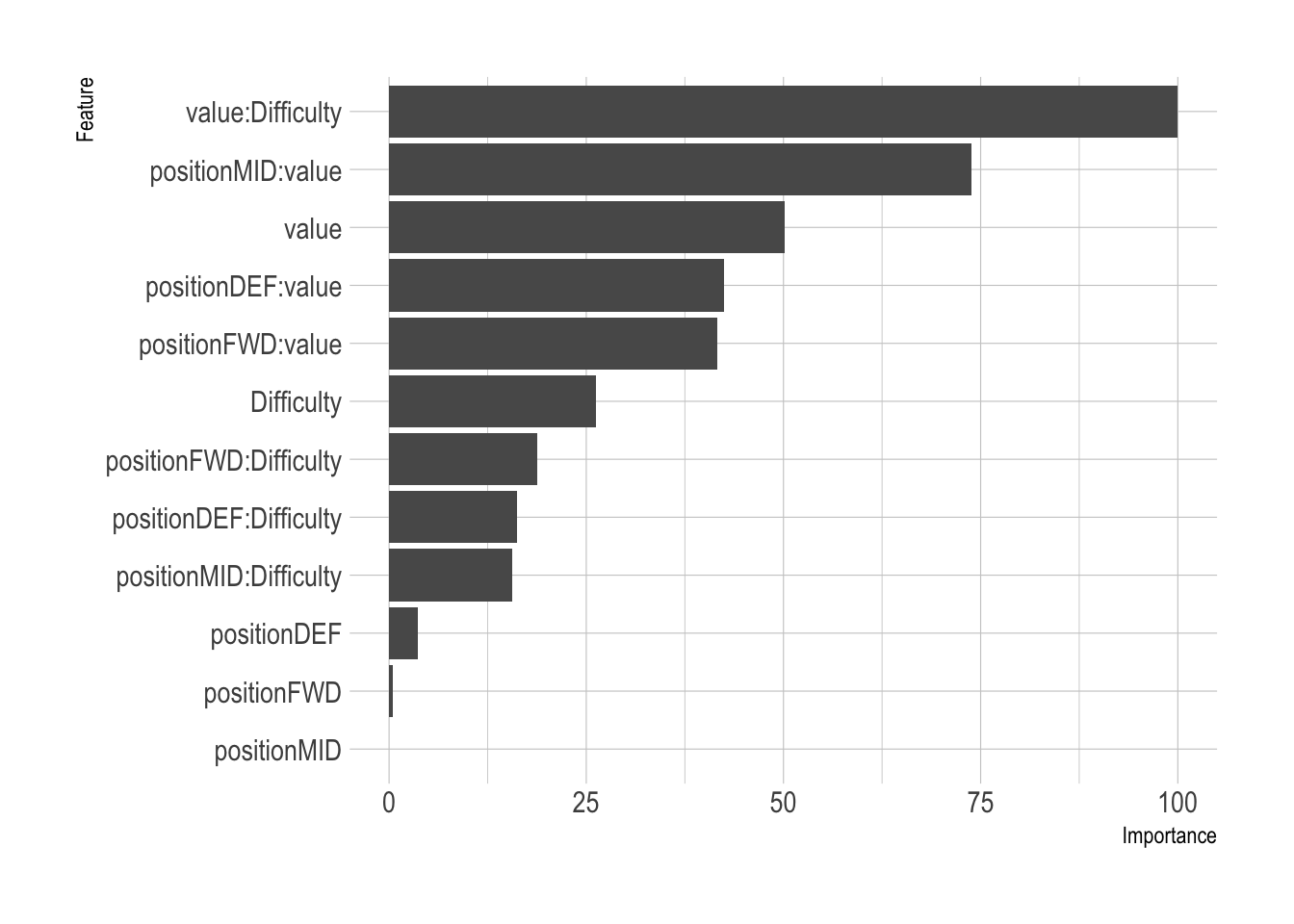
The number one predictor in this model is how much the player cost combined with the difficulty of the match, which shows this new difficulty metric is an important feature of prediction. It is more important for midfield and defenders, which again, is similar to what we saw in the GAM results.
Conclusion
Overall, I hope this again has convinced you how the fixture difficulty can be used to help build you FPL side. The general approach of favouring players with easier matches holds true across all position except for goalkeepers, where they might actually be able to pick up more points in a harder match. It would be a brave strategy to always favour the difficult keeper, but if it came down to your last decision it might be enough of a differential to push you up your minileague.
Environment
knitr::opts_chunk$set(warning = FALSE,
                      fig.retina=2)
require(readr)
require(dplyr)
require(tidyr)
require(ggplot2)
require(caret)
require(mgcv)
require(hrbrthemes)
theme_set(theme_ipsum())