Free Finance Data Sets for the Quants

Now and then I am asked how to get started in quant finance and my advice has always been to just get hold of some data and play about with different models. The first step is to get some data and this post takes you through several different sources and hopefully gives you the launchpad to start poking around with financial data.

Enjoy these types of posts? Then you should sign up for my newsletter.

I’ve tried to cover different assets and frequencies to hopefully inspire the various types of quant finance out there.

High-Frequency FX Market Data

My day-to-day job is in FX so naturally, that’s where I think all the best data can be found. TrueFX provides tick-by-tick in milliseconds, so high-frequency data is available for free and across lots of different currencies. So if you are interested in working out how to deal with large amounts of data (1 month of EURUSD is 600MB) efficiently, this source is a good place to start.

As a demo, I’ve downloaded the USDJPY October dataset.

using CSV, DataFrames, DataFramesMeta, Dates, Statistics
using Plots

It’s a big CSV file, so this isn’t the best way to store the data, instead, stick it into a database like QuestDB that are made for time series data.

usdjpy = CSV.read("USDJPY-2023-10.csv", DataFrame,
                 header = ["Ccy", "Time", "Bid", "Ask"])
usdjpy.Time = DateTime.(usdjpy.Time, dateformat"yyyymmdd HH:MM:SS.sss")
first(usdjpy, 4)

4×4 DataFrame

Row	Ccy	Time	Bid	Ask
	String7	DateTime	Float64	Float64
1	USD/JPY	2023-10-01T21:04:56.931	149.298	149.612
2	USD/JPY	2023-10-01T21:04:56.962	149.298	149.782
3	USD/JPY	2023-10-01T21:04:57.040	149.589	149.782
4	USD/JPY	2023-10-01T21:04:58.201	149.608	149.782

It’s simple data, just a bid and ask price with a time stamp.

usdjpy = @transform(usdjpy, :Spread = :Ask .- :Bid, 
                            :Mid = 0.5*(:Ask .+ :Bid), 
                            :Hour = round.(:Time, Minute(10)))

usdjpyHourly = @combine(groupby(usdjpy, :Hour), :open = first(:Mid), :close = last(:Mid), :avg_spread = mean(:Spread))
usdjpyHourly.Time = Time.(usdjpyHourly.Hour)

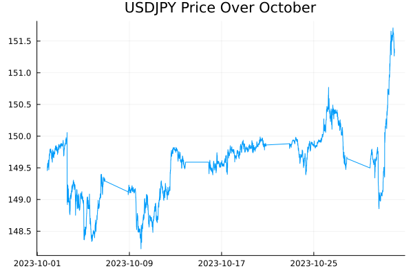
plot(usdjpyHourly.Hour, usdjpyHourly.open, lw =1, label = :none, title = "USDJPY Price Over October")

Looking at the hourly price over the month gives you flat periods over the weekend.

USDJPY October price chart

Let’s look at the average spread (ask - bid) throughout the day.

hourlyAvgSpread = sort(@combine(groupby(usdjpyHourly, :Time), :avg_spread = mean(:avg_spread)), :Time)

plot(hourlyAvgSpread.Time, hourlyAvgSpread.avg_spread, lw =2, title = "USDJPY Intraday Spread", label = :none)

USDJPY average intraday spread

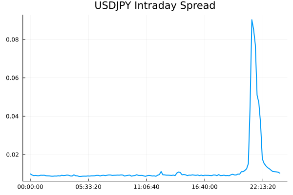
We see a big spike at 10 pm because of the day roll and the secondary markets go offline briefly, which pollutes the data bit. Looking at just midnight to 8 pm gives a more indicative picture.

plot(hourlyAvgSpread[hourlyAvgSpread.Time .<= Time("20:00:00"), :].Time, 
     hourlyAvgSpread[hourlyAvgSpread.Time .<= Time("20:00:00"), :].avg_spread, label = :none, lw=2,
     title = "USDJPY Intraday Spread")

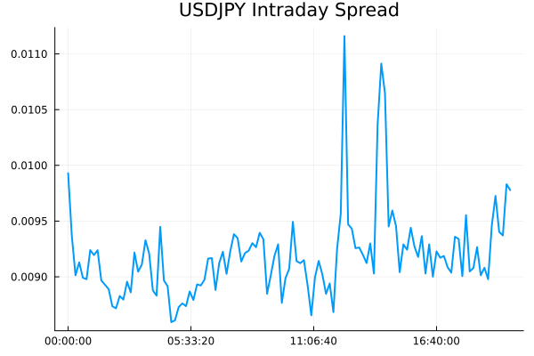
USDJPY average intraday spread zoomed

In October spreads have generally been wider in the later part of the day compared to the morning.

There is much more that can be done with this data across the different currencies though. For example:

How stable are correlations across currencies at different time frequencies?
Can you replicate my microstructure noise post? How does the microstructure noise change between currencies
Price updates are irregular, what are some statistical properties?

Daily Futures Market Data

Let’s zoom out a little bit now, decrease the frequency, and widen the asset pool. Futures cover many asset classes, oil, coal, currencies, metals, agriculture, stocks, bonds, interest rates, and probably something else I’ve missed. This data is daily and roll adjusted, so you have a continuous time series of an asset for many years. This means you can look at the classic momentum/mean reversion portfolio models and have a real stab at long-term trends.

The data is part of the Nasdaq data link product (formerly Quandl) and once you sign up for an account you have access to the free data. This futures dataset is Wiki Continuous Futures and after about 50 clicks and logging in, re-logging in, 2FA codes you can view the pages.

To get the data you can go through one of the API packages in your favourite language. In Julia, this means the QuandlAccess.jl package which keeps things simple.

using QuandlAccess

futuresMeta = CSV.read("continuous.csv", DataFrame)
futuresCodes = futuresMeta[!, "Quandl Code"] .* "1"

quandl = Quandl("QUANDL_KEY")

function get_data(code)
    futuresData = quandl(TimeSeries(code))
    futuresData.Code .= code
    futuresData
end
futureData = get_data.(rand(futuresCodes, 4));

We have an array of all the available contracts futuresCodes and sample 4 of them randomly to see what the data looks like.

p = []
for df in futureData
    append!(p, plot(df.Date, df.Settle, label = df.Code[1]))
end

plot(plot.(p)..., layout = 4)

Futures examples

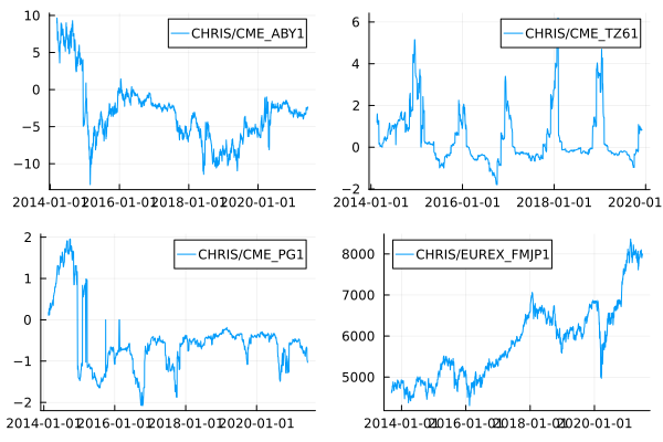
ABY - WTI Brent Bullet - Spread between two oil futures on different exchanges.
TZ6 - Transco Zone 6 Non-N.Y. Natural Gas (Platts IFERC) Basis - Spread between two different natural gas contracts
PG - PG&E Citygate Natural Gas (Platts IFERC) Basis - Again, spread between two different natural gas contracts
FMJP - MSCI Japan Index - Index containing Japanese stocks

I’ve managed to randomly select 3 energy futures and one stock index.

Project ideas with this data:

Cross-asset momentum and mean reversion.
Cross-asset correlations, does the price of oil drive some equity indexes?
Macro regimes, can you pick out commonalities of market factors over the years?

Equity Order Book Data

Out there in the wild is the FI2010 dataset which is essentially a sample of the full order book for five different stocks on the Nordic stock exchange for 10 days. You have 10 levels of prices and volumes and so can reconstruct the order book throughout the day. It is the benchmark dataset for limit order book prediction and you will see it referenced in papers that are trying to implement new prediction models. For example Benchmark Dataset for Mid-Price Forecasting of Limit Order Book Data with Machine Learning Methods references some basic methods on the dataset and how they perform when predicting the mid-price.

I found the dataset (as a Python package) here https://github.com/simaki/fi2010 but it’s just stored as a CSV which you can lift easily.

fi2010 = CSV.read(download("https://raw.githubusercontent.com/simaki/fi2010/main/data/data.csv"),DataFrame);

Update on 7/01/2024

Since posting this the above link has gone offline and the user has deleted their Github account! Instead the data set can be found here: https://etsin.fairdata.fi/dataset/73eb48d7-4dbc-4a10-a52a-da745b47a649/data . I’ve not verified if its in the same format, so there might be some additional work going from the raw data to how this blog post sets it up. Thank’s to the commentators below pointing this out.

The data is wide (each column is a depth level of the price and volume) so I turn each into a long data set and add the level, side and variable as a new column.

fi2010Long = stack(fi2010, 4:48, [:Column1, :STOCK, :DAY])
fi2010Long = @transform(fi2010Long, :a = collect.(eachsplit.(:variable, "_")))
fi2010Long = @transform(fi2010Long, :var = first.(:a), :level = last.(:a), :side = map(x->x[2], :a))
fi2010Long = @transform(groupby(fi2010Long, [:STOCK, :DAY]), :Time = collect(1:length(:Column1)))
first(fi2010Long, 4)

The ‘book depth’ is the sum of the liquidity available at all the levels and indicates how easy it is to trade the stock. As a quick example, we can take the average of each stock per day and use that as a proxy for the ease of trading these stocks.

intraDayDepth = @combine(groupby(fi2010Long, [:STOCK, :DAY, :var]), :avgDepth = mean(:value))
intraDayDepth = @subset(intraDayDepth, :var .== "VOLUME");
plot(intraDayDepth.DAY, intraDayDepth.avgDepth, group=intraDayDepth.STOCK, 
     marker = :circle, title = "Avg Daily Book Depth - FI2010")

FI2010 Intraday book depth

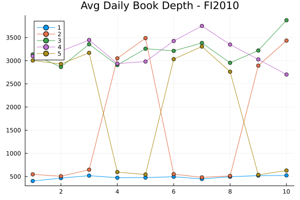
Stock 3 and 4 have the highest average depth, so most likely the easier to trade, whereas Stock 1 has the thinnest depth. Stock 2 has an interesting switch between liquid and not liquid.

So if you want to look beyond top-of-book data, this dataset provides the extra level information needed and is closer to what a professional shop is using. Better than trying to predict daily Yahoo finance mid-prices with neural nets at least.

Build Your Own Crypto Datasets

If you want to take a further step back then being able to build the tools that take in streaming data directly from the exchanges and save that into a database is another way you can build out your technical capabilities. This means you have full control over what you download and save. Do you want just the top of book every update, the full depth of the book, or just the reported trades? I’ve written about this before, Getting Started with High Frequency Finance using Crypto Data and Julia, and learned a lot in the process. Doing things this way means you have full control over the entire process and can fully understand the data you are saving and any additional quirks around the process.

Conclusion

Plenty to get stuck into and learn from. Being able to get the data and loading it into an environment is always the first challenge and learning how to do that with all these different types of data should help you understand what these types of jobs entail.