Calibrating an Ornstein–Uhlenbeck Process
Read enough quant finance papers or books and you’ll come across the Ornstein–Uhlenbeck (OU) process. This is a post that explores the OU process, the equations, how we can simulate such a process and then estimate the parameters.
Enjoy these types of posts? Then you should sign up for my newsletter.
I’ve briefly touched on mean reversion and OU processes before in my Stat Arb - An Easy Walkthrough blog post where we modelled the spread between an asset and its respective ETF. The whole concept of ‘mean reversion’ is something that comes up frequently in finance and at different time scales. It can be thought of as the first basic extension as Brownian motion and instead of things moving randomly there is now a slight structure where it be oscillating around a constant value.
The Hudson Thames group have a similar post on OU processes (Mean-Reverting Spread Modeling: Caveats in Calibrating the OU Process) and my post should be a nice compliment with code and some extensions.
The Ornstein-Uhlenbeck Equation
As a continuous process, we write the change in \(X_t\) as an increment in time and some noise
\[\mathrm{d}X_t = \theta (\mu - x_t) \mathrm{d}t + \sigma \mathrm{d}W_t\]The amount it changes in time depends on the previous \(X_t\) and to free parameters \(\mu\) and \(\theta\).
- The \(\mu\) is the long-term drift of the process
- The \(\theta\) is the mean reversion or momentum parameter depending on the sign.
If \(\theta\) is 0 we can see the equation collapses down to a simple random walk.
If we assume \(\mu = 0\), so the long-term average is 0, then a positive value of \(\theta\) means we see mean reversion. Large values of \(X\) mean the next change is likely to have a negative sign, leading to a smaller value in \(X\).
A negative value of \(\theta\) means the opposite and we end up with a large value in X generating a further large positive change and the process explodes. E If discretise the process we can simulate some samples with different parameters to illustrate these two modes.
\[X_{t+1} - X_t = \theta (\mu - X_t) \Delta t + \sigma \sqrt{\Delta t} W_t\]where \(W_t \sim N(0,1)\).
which is easy to write out in Julia. We can save some time by drawing the random values first and then just summing everything together.
using Distributions, Plots

function simulate_os(theta, mu, sigma, dt, maxT, initial)
    p = Array{Float64}(undef, length(0:dt:maxT))
    p[1] = initial
    w = sigma * rand(Normal(), length(p)) * sqrt(dt)
    for i in 1:(length(p)-1)
        p[i+1] = p[i] + theta*(mu-p[i])*dt + w[i]
    end
    return p
end
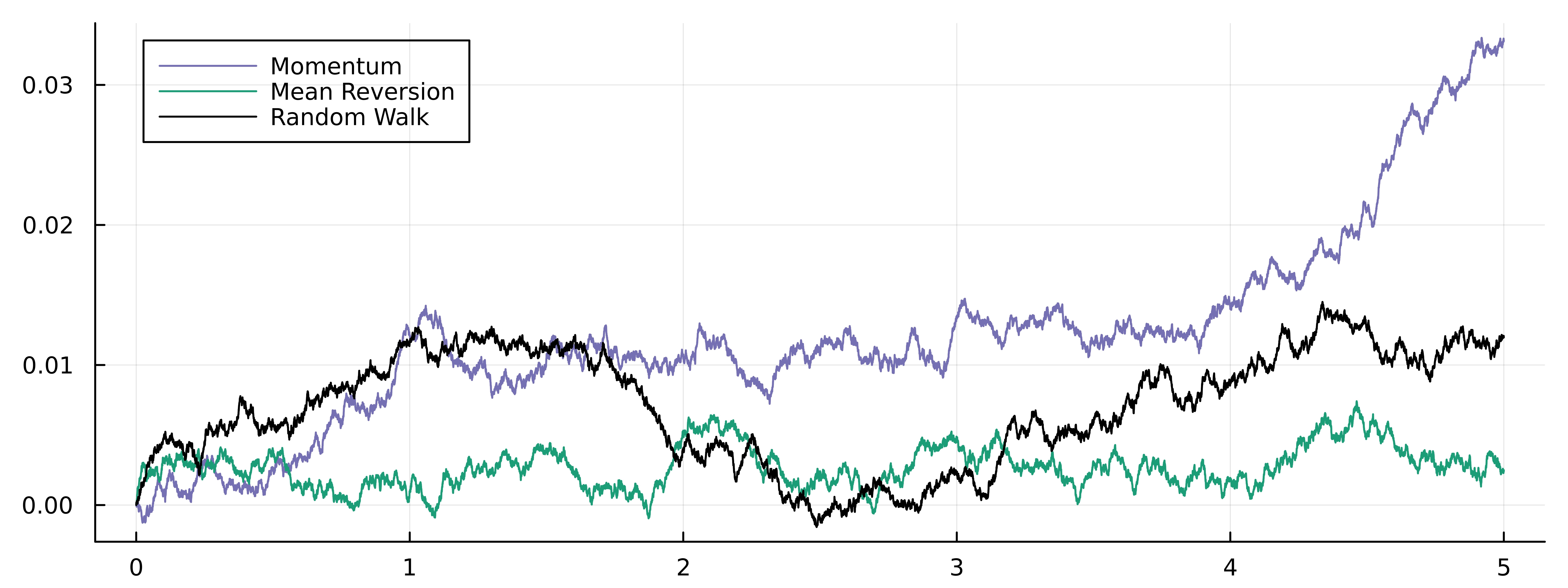
We have two classes of OU processes we want to simulate, a mean reverting \(\theta > 0\) and a momentum version (\(\theta < 0\)) and we also want to simulate a random walk at the same time, so \(\theta = 0\). We will assume \(\mu = 0\) which keeps the pictures simple.
maxT = 5
dt = 1/(60*60)
vol = 0.005

initial = 0.00*rand(Normal())

p1 = simulate_os(-0.5, 0, vol, dt, maxT, initial)
p2 = simulate_os(0.5, 0, vol, dt, maxT, initial)
p3 = simulate_os(0, 0, vol, dt, maxT, initial)

plot(0:dt:maxT, p1, label = "Momentum")
plot!(0:dt:maxT, p2, label = "Mean Reversion")
plot!(0:dt:maxT, p3, label = "Random Walk")

The mean reversion (orange) hasn’t moved away from the long-term average (\(\mu=0\)) and the momentum has diverged the furthest from the starting point, which lines up with the name. The random walk, inbetween both as we would expect.
Now we have successfully simulated the process we want to try and estimate the \(\theta\) parameter from the simulation. We have two slightly different (but similar methods) to achieve this.
OLS Calibration of an OU Process
When we look at the generating equation we can simply rearrange it into a linear equation.
\[\Delta X = \theta \mu \Delta t - \theta \Delta t X_t + \epsilon\]and the usual OLS equation
\[y = \alpha + \beta X + \epsilon\]such that
\[\alpha = \theta \mu \Delta t\] \[\beta = -\theta \Delta t\]where \(\epsilon\) is the noise. So we just need a DataFrame with the difference between subsequent observations and relate that to the current observation. Just a diff and a shift.
using DataFrames, DataFramesMeta
momData = DataFrame(y=p1)
momData = @transform(momData, :diffY = [NaN; diff(:y)], :prevY = [NaN; :y[1:(end-1)]])
Then using the standard OLS process from the GLM package.
mdl = lm(@formula(diffY ~ prevY), momData[2:end, :])
alpha, beta = coef(mdl)

theta = -beta / dt
mu = alpha / (theta * dt)
Which gives us \(\mu = 0.0075, \theta = -0.3989\), so close to zero for the drift and the reversion parameter has the correct sign.
Doing the same for the mean reversion data.
mdl = lm(@formula(diffY ~ prevY), revData[2:end, :])
alpha, beta = coef(mdl)

theta = -beta / dt
mu = alpha / (theta * dt)
This time \(\mu = 0.001\) and \(\theta = 1.2797\). So a little wrong compared to the true values, but at least the correct sign.
Does Bootstrapping Help?
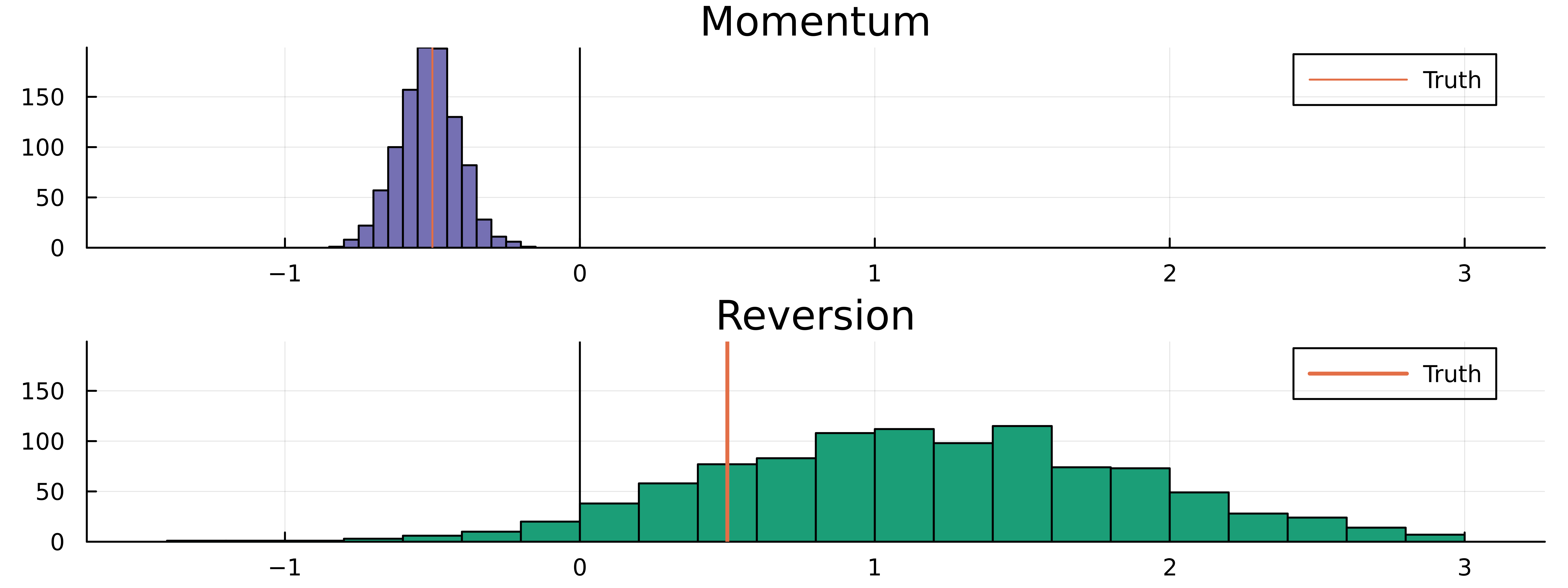
It could be that we need more data, so we use the bootstrap to randomly sample from the population to give us pseudo-new draws. We use the DataFrames again and pull random rows with replacement to build out the data set. We do this sampling 1000 times.
res = zeros(1000)
for i in 1:1000
    mdl = lm(@formula(diffY ~ prevY + 0), momData[sample(2:nrow(momData), nrow(momData), replace=true), :])
    res[i] = -first(coef(mdl)/dt)
end

bootMom = histogram(res, label = :none, title = "Momentum", color = "#7570b3")
bootMom = vline!(bootMom, [-0.5], label = "Truth", momentum = 2)
bootMom = vline!(bootMom, [0.0], label = :none, color = "black")
We then do the same for the reversion data.
res = zeros(1000)
for i in 1:1000
    mdl = lm(@formula(diffY ~ prevY + 0), revData[sample(2:nrow(revData), nrow(revData), replace=true), :])
    res[i] = first(-coef(mdl)/dt)
end

bootRev = histogram(res, label = :none, title = "Reversion", color = "#1b9e77")
bootRev = vline!(bootRev, [0.5], label = "Truth", lw = 2)
bootRev = vline!(bootRev, [0.0], label = :none, color = "black")
Then combining both the graphs into one plot.
plot(bootMom, bootRev,
  layout=(2,1),dpi=900, size=(800, 300),
  background_color=:transparent, foreground_color=:black,
     link=:all)

The momentum bootstrap has worked and centred around the correct value, but the same cannot be said for the reversion plot. However, it has correctly guessed the sign.
AR(1) Calibration of a OU Process
If we continue assuming that \(\mu = 0\) then we can simplify the OLS to a 1-parameter regression - OLS without an intercept. From the generating process, we can see that this is an AR(1) process - each observation depends on the previous observation by some amount.
\[\phi = \frac{\sum _i X_i X_{i-1}}{\sum _i X_{i-1}^2}\]then the reversion parameter is calculated as
\[\theta = - \frac{\log \phi}{\Delta t}\]This gives us a simple equation to calculate \(\theta\) now.
For the momentum sample:
phi = sum(p1[2:end] .* p1[1:(end-1)]) / sum(p1[1:(end-1)] .^2)
-log(phi)/dt
Givens \(\theta = -0.50184\), so very close to the true value.
For the reversion sample
phi = sum(p2[2:end] .* p2[1:(end-1)]) / sum(p2[1:(end-1)] .^2)
-log(phi)/dt
Gives \(\theta = 1.26\), so correct sign, but quite a way off.
Finally, for the random walk
phi = sum(p3[2:end] .* p3[1:(end-1)]) / sum(p3[1:(end-1)] .^2)
-log(phi)/dt
Produces \(\theta = -0.027\), so quite close to zero.
Again, values are similar to what we expect, so our estimation process appears to be working.
Using Multiple Samples for Calibrating an OU Process
If you aren’t convinced I don’t blame you. Those point estimates above are nowhere near the actual values that simulated the data so it’s hard to believe the estimation method is working. Instead, what we need to do is repeat the process and generate many more price paths and estimate the parameters of each one.
To make things a bit more manageable code-wise though I’m going to
introduce a struct that contains the parameters and allows to
simulate and estimate in a more contained manner.
struct OUProcess
    theta
    mu
    sigma
    dt
    maxT
    initial
end
We now write specific functions for this object and this allows us to simplify the code slightly.
function simulate(ou::OUProcess)
    simulate_os(ou.theta, ou.mu, ou.sigma, ou.dt, ou.maxT, ou.initial)
end

function estimate(ou::OUProcess)
   p = simulate(ou)
   phi =  sum(p[2:end] .* p[1:(end-1)]) / sum(p[1:(end-1)] .^2)
   -log(phi)/ou.dt
end

function estimate(ou::OUProcess, N)
    res = zeros(N)
    for i in 1:N
        p = simulate(ou)
        res[i] = estimate(ou)
    end
    res
end
We use these new functions to draw from the process 1,000 times and sample the parameters for each one, collecting the results as an array.
ou = OUProcess(0.5, 0.0, vol, dt, maxT, initial)
revPlot = histogram(estimate(ou, 1000), label = :none, title = "Reversion")
vline!(revPlot, [0.5], label = :none);
And the same for the momentum OU process
ou = OUProcess(-0.5, 0.0, vol, dt, maxT, initial)
momPlot = histogram(estimate(ou, 1000), label = :none, title = "Momentum")
vline!(momPlot, [-0.5], label = :none);
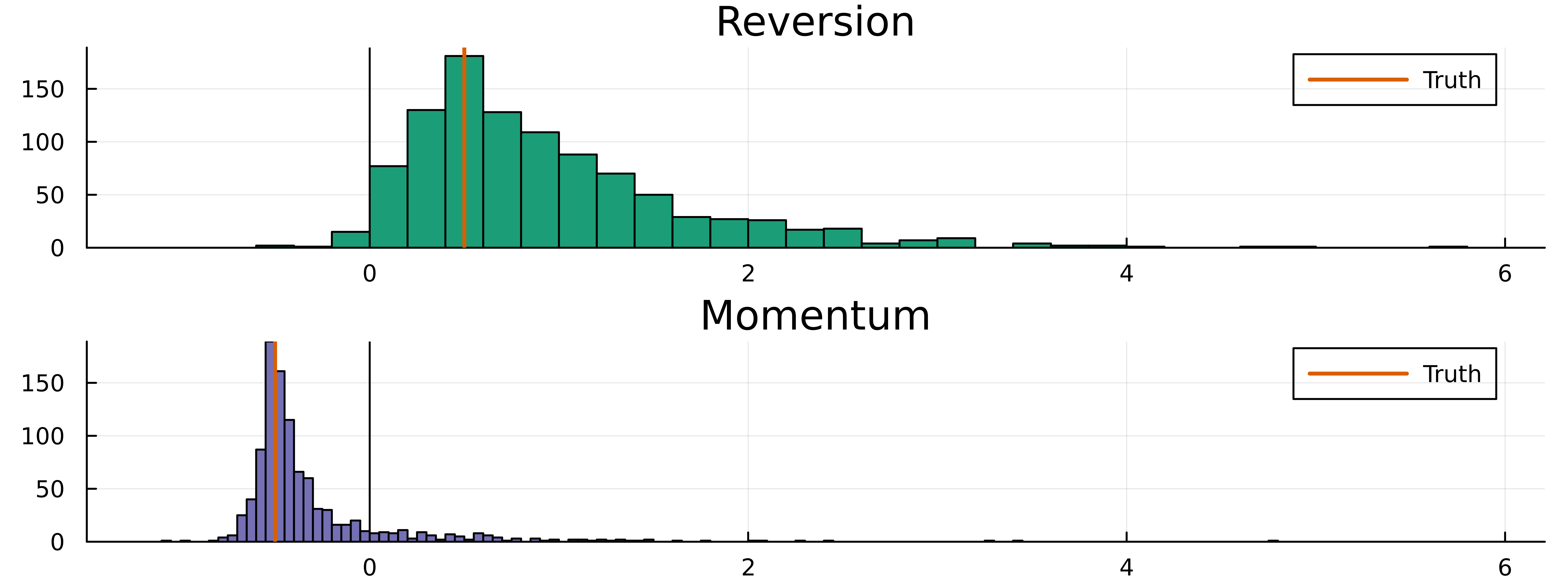
Plotting the distribution of the results gives us a decent understanding of how varied the samples can be.
plot(revPlot, momPlot, layout = (2,1), link=:all)

We can see the heavy-tailed nature of the estimation process, but thankfully the histograms are centred around the correct number. This goes to show how difficult it is to estimate the mean reversion parameter even in this simple setup. So for a real dataset, you need to work out how to collect more samples or radically adjust how accurate you think your estimate is.
Summary
We have progressed from simulating an Ornstein-Uhlenbeck process to estimating its parameters using various methods. We attempted to enhance the accuracy of the estimates through bootstrapping, but we discovered that the best approach to improve the estimation is to have multiple samples.
So if you are trying to fit this type of process on some real world data, be it the spread between two stocks (Statistical Arbitrage in the U.S. Equities Market), client flow (Unwinding Stochastic Order Flow: When to Warehouse Trades) or anything else you believe might be mean reverting, then understand how much data you might need to accurately model the process.