Predicting Goals Using the Winning Odds
The odds of a football match is the market’s view of how that match will play out. We want to use this one price to try and predict other features of the match, in this case, how many goals a team will score.
Enjoy these types of posts? Then sign up for my newsletter.
Following on from my Hawkes processes and terrorist attacks post, this is a further look into my Ph.D. dissertation and another chapter of my research. This will be a two-parter of a blog post, firstly, this one will deal with predicting how many goals a team will score based on the probability that they will win the match. The second post will then look at where these goals are distributed through the game and build a nice non-parametric model for this “goal intensity curve”.
The underlying model driving a teams goal scoring can be written as:
\[p(\text{goal}) = \Lambda \cdot f(t),\]where \(\Lambda\) is the estimated number of goals that they might score, and \(f(t)\) is a density over the duration of the match when they might score them. So hopefully you can see why this type of model can be separated into two components and thus two blog posts.
- First we build a model for \(\Lambda\) using Poisson regression.
- We model \(f(t)\) using a Dirichlet process.
This post will be looking at part 1 and how we approach the modeling. I’ll be fitting different models, comparing their performance, and showing you how to then upgrade the model to a Bayesian version.
My R Environment
To follow along you will need these packages.
knitr::opts_chunk$set(fig.retina=2)
require(readr)
require(dplyr)
require(tidyr)
require(ggplot2)
require(rstanarm)
require(mgcv)
require(caret)
require(lubridate)
The Football Data
Like all of my football posts, the data comes from
https://www.football-data.co.uk/. I will be using the FTG column and
the Pinnacle sports closing odds columns (PSCH, PSCD, PSCA) to
calculate the probability a team was going to win a match. This
probability contains the best estimate of a team’s strength right up
until the point they kick-off, so it saves us having to take into
account recent form, injuries, and things like that.
fn <- list.files("~/Documents/Programming/Ref Data/Betting/BulkData/BulkData/", full.names = T)
rawDataList <- lapply(fn, read_csv, guess_max=10000))
rawData <- bind_rows(rawDataList)
rm(rawDataList)
With the data loaded we now want to wrangle it into a more convenient format.
rawData %>%
  select(Div, Date, HomeTeam, AwayTeam,
         FTHG, FTAG, HTHG, HTAG,
         PSCH, PSCA, PSCD) %>%
  drop_na -> cleanData

cleanData %>%
  select(Div, Date, HomeTeam, FTHG, HTHG, PSCH, PSCA, PSCD) %>%
  rename(Team = HomeTeam, FTG = FTHG, HTG = HTHG,
         WinOdds = PSCH, LoseOdds = PSCA, DrawOdds = PSCD) %>%
  mutate(Home = 1) -> homeData

cleanData %>%
  select(Div, Date, AwayTeam, FTAG, HTAG, PSCH, PSCA, PSCD) %>%
  rename(Team = AwayTeam, FTG = FTAG, HTG = HTAG,
         WinOdds = PSCA, LoseOdds = PSCH, DrawOdds = PSCD) %>%
  mutate(Home = 0) -> awayData

allData <- bind_rows(homeData, awayData)
allData %>%
  mutate(WinProbRaw = 1/WinOdds,
         LoseProbRaw = 1/LoseOdds,
         DrawProbRaw = 1/DrawOdds,
         WinProb = WinProbRaw /(WinProbRaw + LoseProbRaw + DrawProbRaw),
         LoseProb = LoseProbRaw /(WinProbRaw + LoseProbRaw + DrawProbRaw),
         DrawProb = DrawProbRaw /(WinProbRaw + LoseProbRaw + DrawProbRaw),
         Date = dmy(Date)) -> allData
Each match consists of two teams, so we can double up the size of the data by taking each team, their odds of winning, and the number of goals they scored. To calculate the winning probability, we take the inverse of the odds and then normalise it by the summation of the three outcomes, this removes the over round and also ensures the probabilities add up to one.
The final data looks like this:
- Descriptive variables
- Division, Date, Team, and if they were at home.
- Odds
- The raw odds are taken from the Pinnacle closing odds.
- Probabilities
- Converting the odds to winning probabilities by removing the over-round.
We can now set up the classic train/test split by using the
createDataPartition function from caret.
trainInds <- createDataPartition(allData$Div, p = 0.7, list=FALSE)

trainData <- allData[trainInds, ]
testData <- allData[-trainInds, ]
This gives us 71259 observations to train on and 30527 to test on.
Null Model
Our null model is just the average number of goals scored across the training set.
nullModel <- glm(FTG ~ 1, data=trainData, family="poisson")
Linear Model
We now update the null model to include the win probability as a single predictor.
winOddsModel <- glm(FTG ~ WinProb, family = "poisson", data=trainData)
4th Order Polynomial Model
We now include multiple powers of the win probability, up to the 4th power.
winOddsPolyModel <- glm(FTG ~ WinProb +
                          I(WinProb^2) +
                          I(WinProb^3) +
                          I(WinProb^4), family = "poisson",
                        data=trainData)
GAM
Finally, we fit a GAM, so look at the full nonlinear response of the win probability to the number of goals.
require(mgcv)
winOddsGAMModel <- gam(FTG ~ s(WinProb), family="poisson",
                       data=trainData)
Comparing Models
We can visualise the models by plotting the expected number of goals across a grid of different win probabilities.
oddsGrid <- data.frame(WinProb=seq(0, 1, by=0.01))
oddsShape <- predict(winOddsModel, newdata = oddsGrid)
polyShape <- predict(winOddsPolyModel, newdata = oddsGrid)
gamShape <- predict(winOddsGAMModel, newdata = oddsGrid)
nullShape <- predict(nullModel, newdata = oddsGrid)

oddsGrid %>%
  mutate(Linear = oddsShape,
         Polynomial = polyShape,
         GAM = gamShape,
         Null = nullShape) -> oddsGrid

oddsGrid %>% gather(Model, Value, -WinProb) -> oddsGridTidy
We will compare the shapes to the number of goals in the test set, splitting the different win probabilities into 100 quantiles and calculating the average number of goals.
testData %>%
  group_by(WinProbBucket = cut(WinProb, breaks = seq(0, 1, by=0.01))) %>%
  summarise(N=n(),
            ActualGoals = mean(FTG),
            AvgWinProb = mean(WinProb)) %>%
  ungroup %>% mutate(Model = "Emperical") -> sumData

ggplot() +
  geom_line(data = oddsGridTidy, aes(x=WinProb, y=exp(Value), colour=Model)) +
  geom_point(data=sumData, aes(x=AvgWinProb, y=ActualGoals, colour=Model, alpha=scale(N)), size=2, show.legend = F) +
  theme(legend.position = "bottom", legend.title = element_blank()) +
  ylab("Number of Goals") +
  xlab("Probability of Winning")
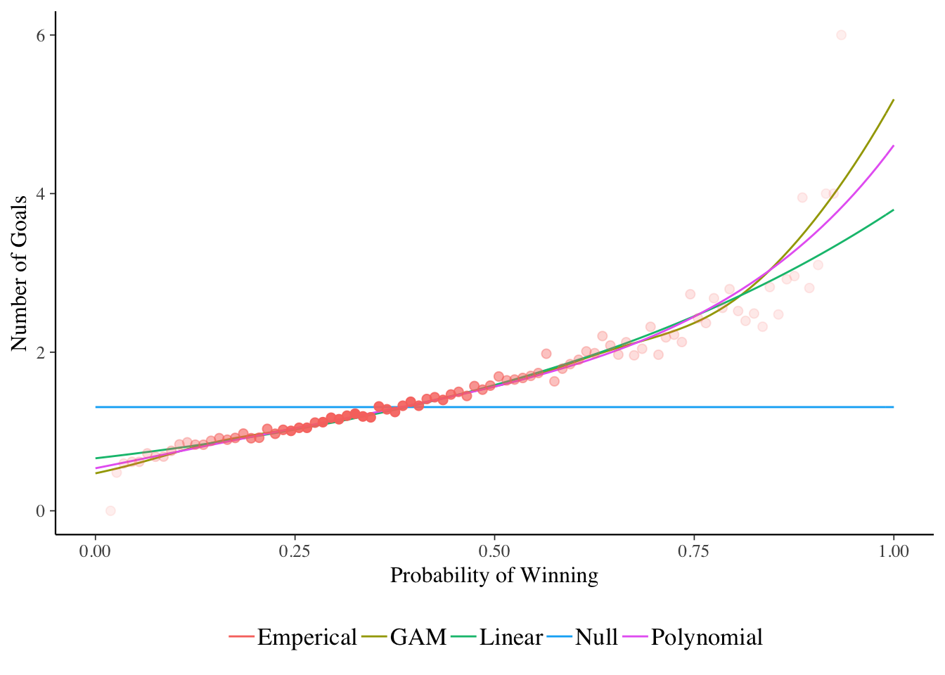
The red dots are the number of goals from the test set, with the fill of the dots indicating how many data points are in the calculation. More solid colour means more games.
We can see the null model just predicting around 1.5 goals per game, the linear model increasing but not quite fast enough for the 0.75+ winning odds. But the GAM and polynomial model fall in line with the data quite nicely.
What Model is Better?
We turn to the next step in working out which model is better. For this I will be using calculating the log-likelihood over the test set and selecting whichever model produces the largest likelihood value.
modelList <- list(NullModel = nullModel,
                  WinOdds = winOddsModel,
                  WinOddsPoly = winOddsPolyModel,
                  WinOddsGAM = winOddsGAMModel)

modelNames <- c("Null", "Linear", "Poly", "GAM")
lambdas <- lapply(modelList,
                  function(x) exp(predict(x, newdata=testData)))
logLikelihoodTest <- lapply(lambdas,
                            function(x) sum(dpois(testData$FTG, x, log = T)))

logLikelihoodTestFrame <- data.frame(Model = modelNames,
                                     LogLikelihoods = unlist(logLikelihoodTest),
                                     Parameters = nrow(trainData) - vapply(modelList, df.residual, numeric(1)))

logLikelihoodTestFrame %>%
  arrange(-LogLikelihoods)
##              Model LogLikelihoods Parameters
## WinOddsGAM     GAM      -43858.09   9.300643
## WinOddsPoly   Poly      -43860.65   5.000000
## WinOdds     Linear      -43861.32   2.000000
## NullModel     Null      -45448.23   1.000000
The GAM has the best likelihood, but the jump from 5 to 8.5 parameters only leads to an improvement of 1.3 on the log-likelihood. This fact, combined with the similar shapes in the above plot suggests that we can get away with the polynomial model.
Fitting a Bayesian Poisson Model
When it comes to fitting the next part of the model when the goals are
scored in the match, we will be using a Bayesian nonparametric method.
So we need to also convert our \(\Lambda\) model to a Bayesian one. This is
simple using the rstanarm package. So rather than approaching all the
other models straight away in a Bayesian manner and potentially wasting
a lot of time waiting for models to compute we can fit them in a
frequentist manner, chose the best one and then refit it using Bayesian
methods.
bayesModel <- stan_glm(FTG ~ WinProb +
                           I(WinProb^2) +
                           I(WinProb^3) +
                           I(WinProb^4),
                         family = "poisson",
                         data=trainData,
                         chains=2)
This the Bayesian model we get the uncertainty around the prediction for free and can see how that lines up with the actual number of goals.
oddsGridBayes <- data.frame(WinProb = seq(0, 1, by=0.01))

linpreds <- posterior_linpred(bayesModel, newdata=oddsGridBayes)

as.data.frame(t(linpreds)) %>%
  mutate(WinProb = oddsGridBayes$WinProb) %>%
  gather(Iteration, Value, -WinProb) %>%
  mutate(ValueExp = exp(Value)) -> linpredsPlot

ggplot(linpredsPlot, aes(x=WinProb, y=ValueExp)) +
  stat_summary(fun.y=mean, geom="line", colour="blue") +
  stat_summary(fun.ymin = function(x) quantile(x, 0.05), fun.ymax = function(x) quantile(x, 0.95), geom="ribbon", alpha=0.5) +
  geom_point(data=sumData, aes(x=AvgWinProb, y=ActualGoals, colour=Model, alpha=scale(N)), size=2, show.legend = F) +
  xlab("Winning Probability") +
  ylab("Number of Goals")
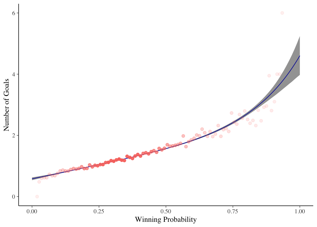
Again, plotting the resulting shape shows a practically identical model that the frequentist model would have found. I’ve also included the 95% credible intervals around the result to give an indication of the uncertainty.
Bayesian Model Checking with Posterior p-values
One of my first blog-post was writing about posterior p-values and how they are used to check a Bayesian model. In short, the number of goals a team would score with each win probability in the data set. This gives us a simulated dataset, which we can then compare to the real training set.
pp_check(bayesModel, plotfun = "ppc_hist", binwidth =1) +
  theme(legend.position = "bottom")
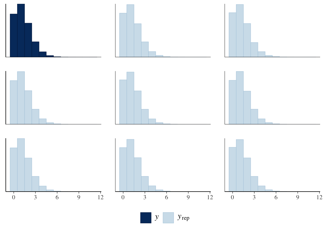
Here each of the light blue facets represents a replicated dataset and solid blue is the actual dataset. We can see that it’s not too bad, our simulated data definitely resembles the actual data. We can then take it a step further and calculate statistics on the replication datasets and compare them to the same statistic on the real data.
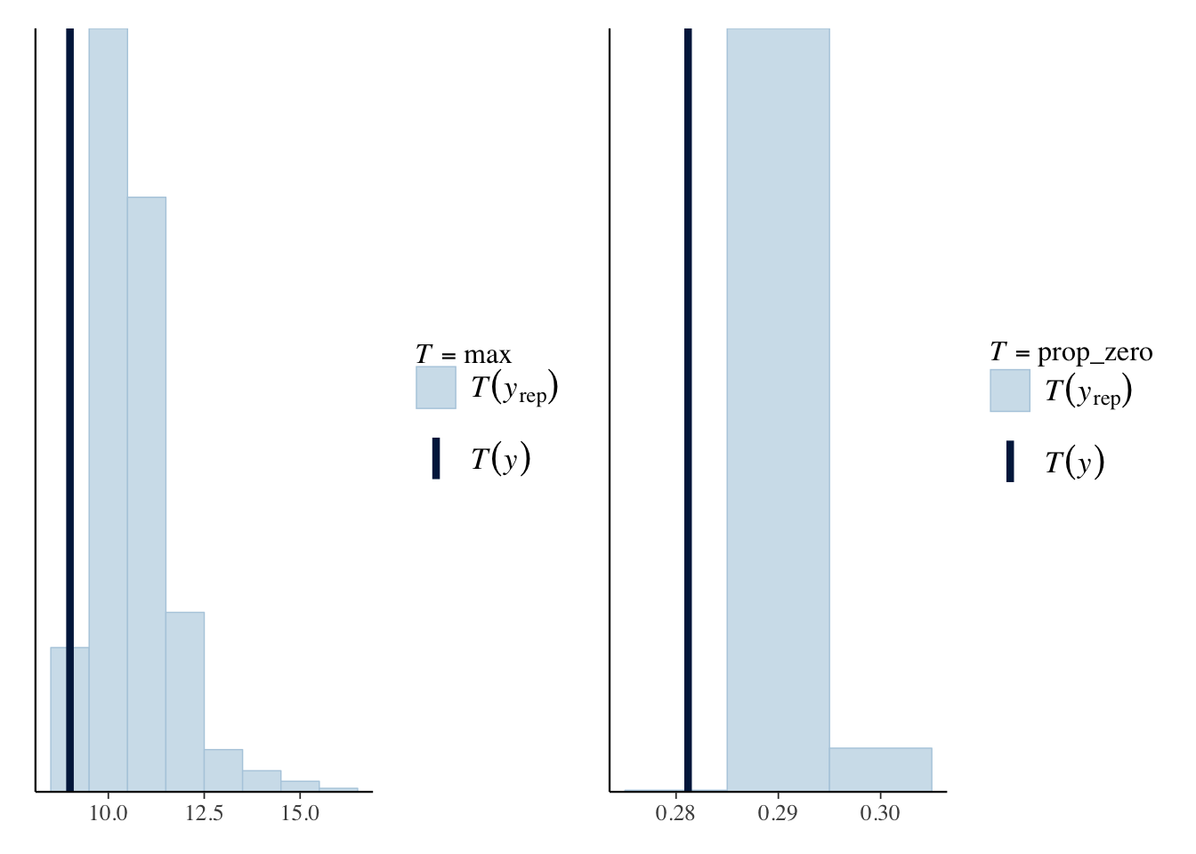
For this example, we will use two statistics, the max and the proportion of matches that had zero goals.
require(patchwork)

prop_zero <- function(x) mean(x == 0)

maxPPC <- pp_check(bayesModel, plotfun = "ppc_stat", stat="max", binwidth=1)
zeroPropPPC <- pp_check(bayesModel, plotfun = "ppc_stat", stat = "prop_zero", binwidth = 0.01)

maxPPC + zeroPropPPC
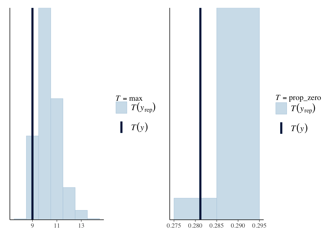
For the max posterior predictive check we can see that our model
slightly over predicts the maximum number of goals, but the real value
of 13 falls in line with the repeated statistics. For the prop_zero
statistic, this also over predicts the proportion of matches with zero
goals and the actual statistic now looks like an outlier to the
repeated distribution.
So some weaknesses in the overall model. How do we remedy this? We can change the family of the regression, to say the negative binomial and see if that helps.
A Negative Binomial Model
The Poisson distributions mean and variance are linked via the same parameter \(\lambda\) which reduces the amount of freedom the model has to fit the data. Whereas the negative binomial distribution has an additional parameter to increase the freedom and potentially fit to the data better.
We switch out the family from poisson to neg_binomial_2. This model
took 5 hours for 500 iterations for 2 chains on 2 cores, so a little
long! You can see why I first fit the models using frequentist methods.
nbModel <- stan_glm(FTG ~ WinProb +
                        I(WinProb^2) +
                        I(WinProb^3) +
                        I(WinProb^4),
                      family = neg_binomial_2,
                      data=trainData,
                      chains=2,
                      cores = 2,
                      iter= 500 )
We go through the same procedure again, looking at the simulated datasets and calculating both the maximum and number of matches with zero goals.
maxPPC_nb <- pp_check(nbModel, plotfun = "ppc_stat", stat="max", binwidth=1)
zeroPropPPC_nb<- pp_check(nbModel, plotfun = "ppc_stat", stat = "prop_zero",
                        binwidth = 0.01)

maxPPC_nb + zeroPropPPC_nb
Unfortunately, it hasn’t fixed the weakness of the Poisson model. So I might as well stick to the simpler Poisson model for our model of \(\Lambda\).
Conclusion
So I fit a number of models that relate the probability of winning to
the number of goals scored. The best-fitting model was a GAM but its
improvement over a 4th order polynomial model wasn’t enough to justify
the extra parameters. I then refit this polynomial model using the
rstanarm package to come up with a Bayesian model. Using posterior-p
values I checked as to whether this model could simulate similar matches
to what the real data resembled. Overall, it was ok, but there was a
minor weakness when looking at the number of zero-goal games. I changed
the model from a Poisson to a negative binomial glm to see if that could
help but this didn’t change the posterior p-values, so we decided to
stick to the Poisson model.
Now this Poisson model is going to feed into the next blog where we model where the goals happen in a game. Stay tuned to learn more about inhomogeneous point processes and how a Dirichlet process can be used in a practical context.
Related Posts
I’ve written similar posts around football: