Easy Neural Nets and Finance - Part 1
I’m fortunate enough to be participating in a lecture series at work that covers deep learning and its applications in finance. This will be a series of posts documenting what I learn and implementing the ‘homework’ (I’m 32, how am I still getting homework?) using Julia and Flux.
Enjoy these types of posts? Then sign up for my newsletter.
The phrase ‘deep learning’ already feels outdated, and the current hotness is more about AI and LLMs, so the lecture and topics might feel a bit out of date. But given LLMs wouldn’t be here without the deep learning, it feels like going back to the basics.
Plus, I’ve never really jumped in and explored neural nets, so this gives me a chance to do some deep learning in an applied way.
After reading this, you will be able to build your own neural net with different layers and compare it to a simpler linear model.
Predicting a Stock’s Daily Volume
If you Google neural nets and finance, you will find an infinite amount of copy-pasted quant finance Python examples of people using PyTorch/TensorFlow/JAX to predict the closing price of some stock. Kudos to these tutorials for putting something out there, but you will struggle to learn anything meaningful about either finance, modelling or neural nets.
This is my attempt to be different.
Instead of predicting prices or returns and showing that neural nets can make money, we will model the total number of shares traded per day. For starters, this is much easier as the data is a bit more signal and less noise. Plus, if I managed to build something that could predict prices, why would I share it?
So, we will be using deep learning to build a model of the total trading volume per day of the SPY ETF. A basic time series prediction task that can be approached both with linear models and deep learning.
You know the drill, fire up your Julia notebook and follow along.
using Dates, AlpacaMarkets, Plots, StatsBase
using DataFramesMeta, ShiftedArrays
Getting the Data
We are using similar data to my Cyclical Embedding post, except for this time, we will be using the SPY ETF instead of Apple.
spyRaw, npt = AlpacaMarkets.stock_bars("SPY", "1Day";
  startTime=Date("2000-01-01"),
  endTime = today() - Day(1) ,
  adjustment = "all", limit = 10000)
From the raw data, we parse the timestamp and scale the volumes by a million.
spy = spyRaw[:, [:t, :v, :c]]
spy[!, "t"] = DateTime.(chop.(spy[!, "t"]));
spy[:, :vNorm] = spy[:, :v] .* 1e-6;
We also add in the returns with a lag because we are using the close-to-close return as a feature.
spy[!, "r"] = log.(spy.c) .- ShiftedArrays.lag(log.(spy.c))
spy[!, "prev_r"] = ShiftedArrays.lag(spy.r);
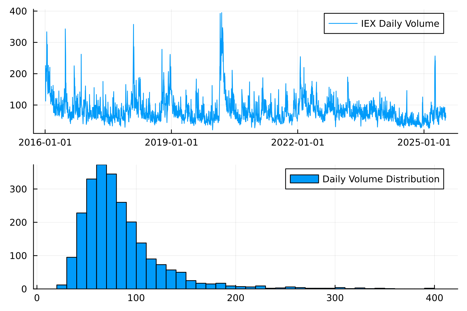
In this data, the daily volume isn’t stationary and it is also heavy-tailed.
plot(
  plot(spy.t, spy.vNorm, label = "IEX Daily Volume"),
  histogram(spy.vNorm, label = "Daily Volume Distribution")
  )
Looking at the autocorrelation, we can see a long-range dependence on the daily volumes, but when we take the daily difference in daily volume, we see a strong effect at lag 1, and the rest are much smaller.
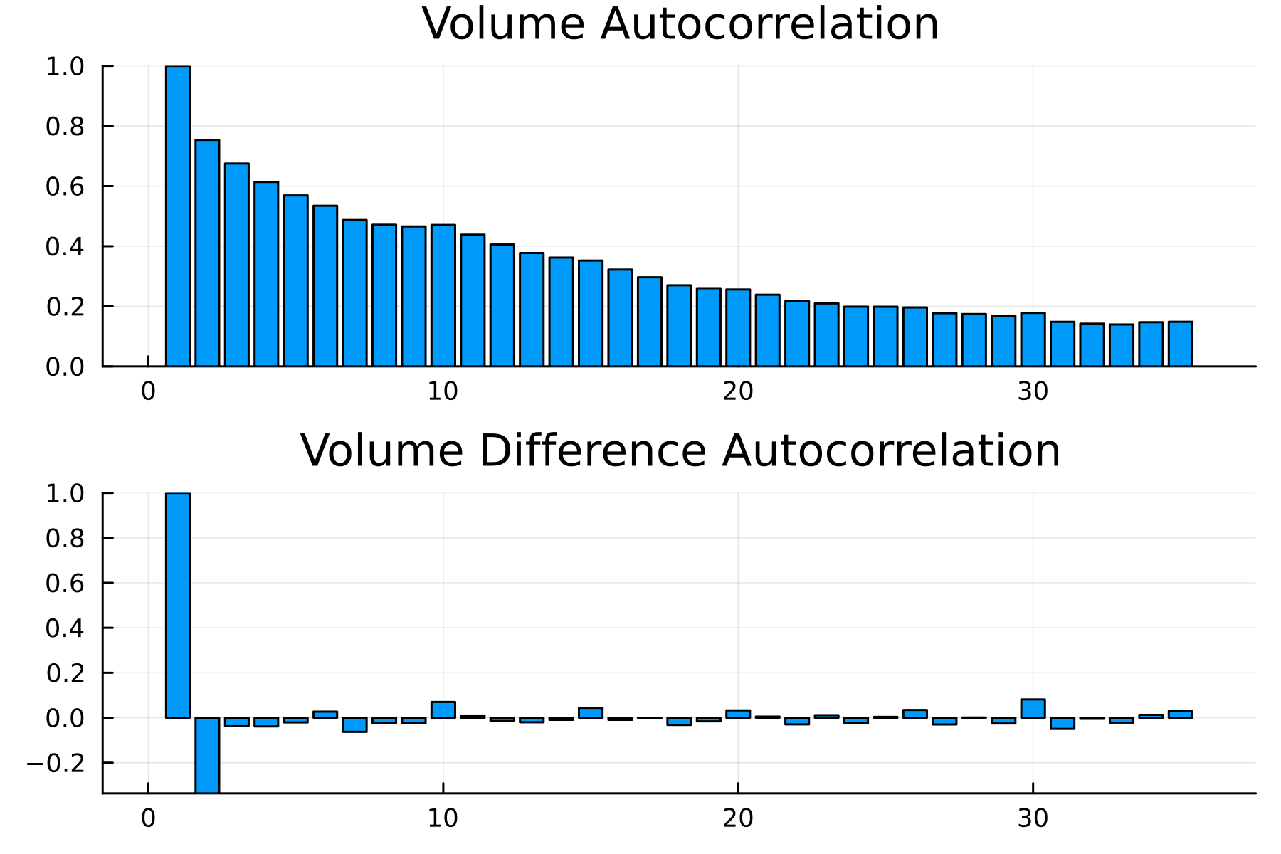
A negative value at lag 1 indicates a mean reversion-like process, but more importantly, means modelling the difference in daily volume will be easier than just directly modelling the daily volumes.
Predicting the daily change in volume does reduce how far out we can forecast volumes, though, as it relies on using the known previous volume to produce the next day’s volume. If you estimate multiple days, then you will be compounding the error.
We lag the volume variables as required.
spy[:, :prev_vNorm] = ShiftedArrays.lag(spy[:, :vNorm])
spy[:, :delta_vNorm] = spy[:, :vNorm] .- spy[:, :prev_vNorm]
spy[:, :prev_delta_vNorm] = ShiftedArrays.lag(spy[:, :delta_vNorm])

spy = dropmissing(spy)
We add in the time-based variables and cyclically encode them.
spy[:, :DayOfMonth] = dayofmonth.(spy.t) .- 1
spy[:, :DayOfWeek] = dayofweek.(spy.t) .- 1
spy[:, :DayOfQtr] = dayofquarter.(spy.t) .- 1
spy[:, :MonthOfYear] = month.(spy.t) .- 1

spy = cyclical_encode(spy, "DayOfWeek")
spy = cyclical_encode(spy, "DayOfMonth")
spy = cyclical_encode(spy, "DayOfQtr")
spy = cyclical_encode(spy, "MonthOfYear");
We also add in if the date was the end of the month.
spy[:, :month] = floor.(spy.t, Dates.Month)
spy = @transform(groupby(spy, :month),
                 :MonthEnd = (:t .== maximum(:t)))
Finally, train/test split.
spyTrain = spy[1:2000, :];
spyTest = spy[2001:end, :];
With the data prepared, we move on to building out the models.
The Baseline Model
We always want to make sure the neural nets are adding value, so we need something simple to compare to. In regular statistical modelling, this might be an intercept-only model, but in this case, we want the best linear model.
It’s a simple linear regression of all the available variables.
using GLM

linearModel = lm(@formula(delta_vNorm ~ prev_delta_vNorm + prev_vNorm +
                                        MonthEnd + prev_r +
                                        DayOfWeek_sin + DayOfWeek_cos +
                                        DayOfMonth_sin + DayOfMonth_cos +
                                        DayOfQtr_sin + DayOfQtr_cos +
                                        MonthOfYear_sin + MonthOfYear_cos
                        ), spyTrain)
This fits instantly and we get an in-sample \(R^2\) of 23% and an out-of-sample MSE of 380.
To add the predicted volume to the test set, we need to add the prediction of the model to the previous volume.
spyTest[!, "linearPred"] = spyTest.prev_vNorm .+ predict(linearModel, spyTest);
sort!(spyTest, :t);

Everything lines up quite nicely. There are a couple of periods where the volume spikes and the model can’t keep up, but other than that, it looks decent.
Also interesting to look at the shape of the cyclically encoded variables.
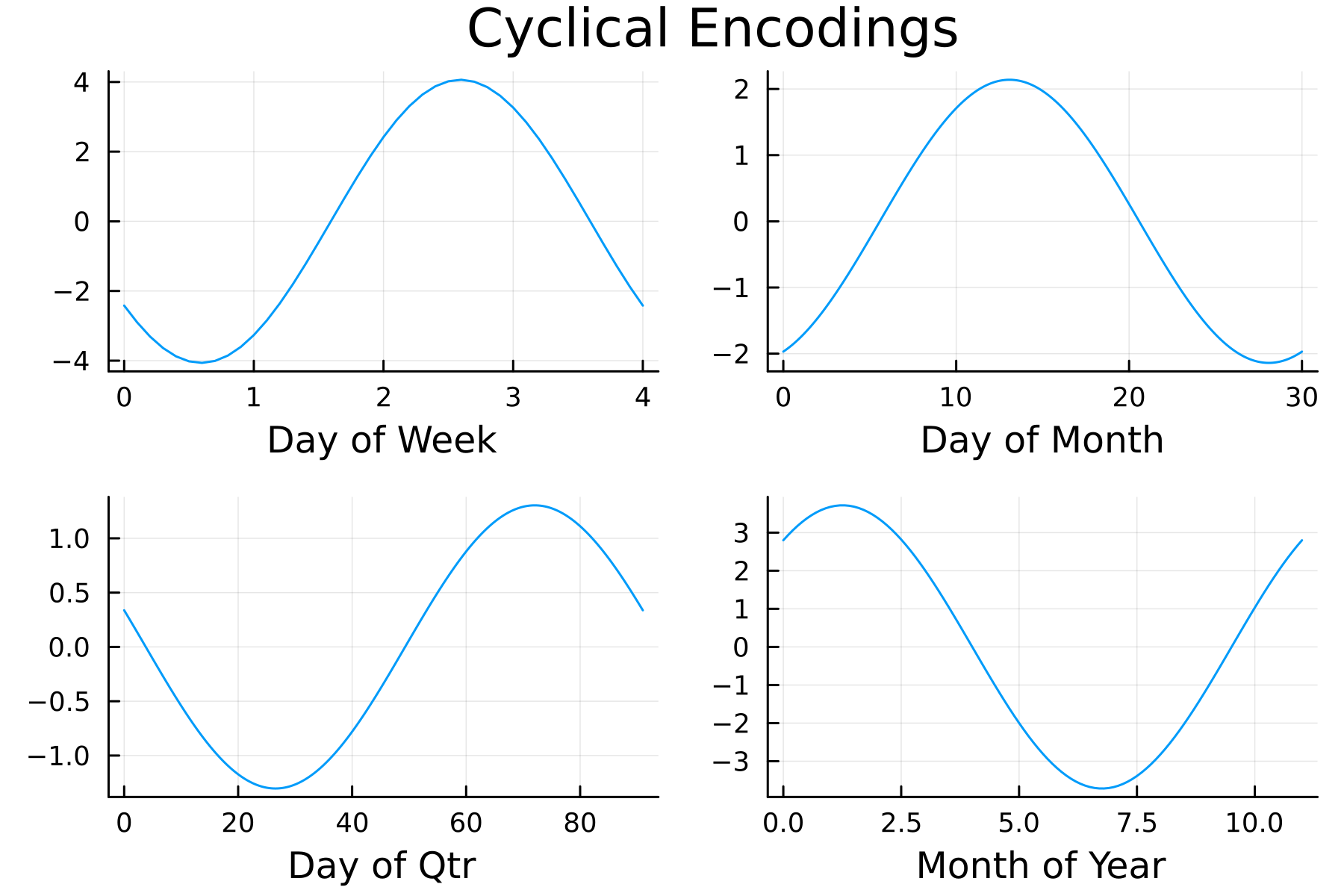
Plenty going on here!
- Day of the Week - Wednesdays and Thursdays have a larger positive effect than Mondays and Tuesdays.
- Day of the Month - The middle of the month (10-15) has the higher positive effect.
- Day of the Quarter - Larger positive effects towards the end of the quarter.
- Month of the Year - Summer months have the most negative effect.
A positive effect here means a larger positive change in the daily volume compared to the previous day, and similarly, the same with the negative effects.
So, an intuitive model to begin with that has produced a strong foundation to improve upon with the neural net models.
Neural Nets in Julia
Let’s increase the model complexity and introduce the neural nets. We are still using the same variables, but we expand them to include even more lags of the change in volumes.
Preparing the Data for a Neural Network
We start with the dataframe, but iterate through and add the 30 lags of the previous volume changes.
rawData = spy[:, [:t, :delta_vNorm, :prev_vNorm, :MonthEnd, :prev_r,
                      :DayOfWeek_sin, :DayOfWeek_cos,
                      :DayOfMonth_sin, :DayOfMonth_cos,
                      :DayOfQtr_sin, :DayOfQtr_cos,
                      :MonthOfYear_sin, :MonthOfYear_cos]]

maxLag = 30
for i in 1:maxLag
    rawData[:, Symbol("lag_$(i)_delta_vNorm")] = ShiftedArrays.lag(rawData.delta_vNorm, i)
end

dropmissing!(rawData)
We then need to go from dataframes to matrices and flip the dimensions so each column is an observation rather than each row.
y = permutedims(rawData.delta_vNorm)
ts = rawData.t
x = @select(rawData, Not(:delta_vNorm, :t))
x = permutedims(Matrix(x));
Again, train/test split too.
xTrain = x[:, 1:2000]
yTrain = y[:, 1:2000]
tsTrain = ts[1:2000]

xTest = x[:, 2001:end]
yTest = y[:, 2001:end]
tsTest = ts[2001:end];
Flux.jl is Julia’s neural network library and the go-to for deep learning in Julia. It provides all the tools to build and train these types of models. One such tool is the DataLoader, which enables batch training for models. Batch training uses random subsets of the full data to train the model, which is very useful if you have too much data to fit into memory. You get to train the model on all your data by breaking it down into chunks.
Now, in this specific case, it isn’t needed as our data is small, but it’s always good to understand the techniques, and Flux makes it very simple. Pass in the x and y matrices, define the batch size and whether you want to randomise the samples or not.
Here we build random batches of 5.
train_loader = Flux.DataLoader((x, y), batchsize=5, shuffle=true);
Next, we need to build the model. In Flux, each layer of the basic net needs the number of input nodes and output nodes.
flux_model = Dense(size(x, 1), 1)
Simply taking the number of rows of the x matrix as the input, and we are outputting 1 number - the expected change in volume for that day.
We also need to define a loss function for the model. We will use the mean square error (MSE). We predict the values from the model and calculate the MSE compared to the true values.
function flux_loss(flux_model, x, y)
    yhat = flux_model(x)
    Flux.mse(yhat, y)
end
A neural net has several parameters that we need to optimise using the training data. With each batch of data, we evaluate the loss function and use the gradient of the loss function to push the parameters in the right direction to minimise the loss. The mechanics of moving around the loss function are controlled by the optimiser. In this case, we will use regular gradient descent, but there are many different optimisers out there that Flux provides - Optimiser Reference.
Again, Flux makes this easy to do out of the box without really needing to understand what’s happening behind the scenes. We provide a gradient descent optimiser, Flux.setup(Descent(eta)), flux_model) (with eta (\(\eta\)) being the learning rate) and update the parameters after each batch of data.
l, gs = Flux.withgradient(m -> flux_loss(m, x, y),flux_model)
Flux.update!(opt_state, flux_model, gs[1])
After all that, we throw everything into one function to easily iterate around the models. We are batch training with gradient descent and returning the trained model plus the loss history on both the full training set and the test set.
function train(train, test, flux_model, flux_loss; batchSize=1024, epochs=10, eta=0.01)
    (xTrain, yTrain) = train
    (xTest, yTest) = test

    train_loader = Flux.DataLoader((xTrain, yTrain), batchsize=batchSize, shuffle=true);
    opt_state = Flux.setup(Descent(eta), flux_model);

    allTrainLoss = zeros(epochs)
    allTestLoss = zeros(epochs)

    for epoch in 1:epochs
        loss = 0.0
        for (x, y) in train_loader
            l, gs = Flux.withgradient(m -> flux_loss(m, x, y), flux_model)
            Flux.update!(opt_state, flux_model, gs[1])
            loss += l / length(train_loader)
        end
        train_loss = flux_loss(flux_model, xTrain, yTrain)
        test_loss = flux_loss(flux_model, xTest, yTest)
        allTrainLoss[epoch] = train_loss
        allTestLoss[epoch] = test_loss

    end
    return (flux_model, allTrainLoss, allTestLoss)
end
We can now train the models, so let’s build some models!
A 1 Layer Neural Net
The simplest neural net is 1 layer with the features as an input and 1 value as the output. Nothing else!
flux_model = Dense(size(x, 1), 1)
flux_model, allTrainLoss, allTestLoss = train((xTrain, yTrain), (xTest, yTest), flux_model, flux_loss; epochs = 1000, eta=1e-6);
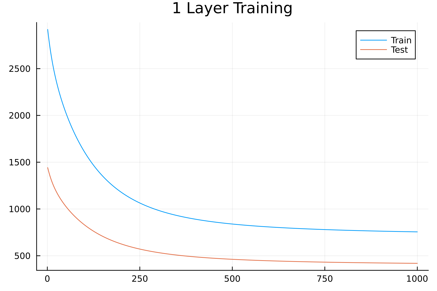
You might notice something strange here: the test loss is smaller than the training loss. This is a quirk of this data set; the test set has a tighter distribution than the training data, which is easy to see in a histogram.
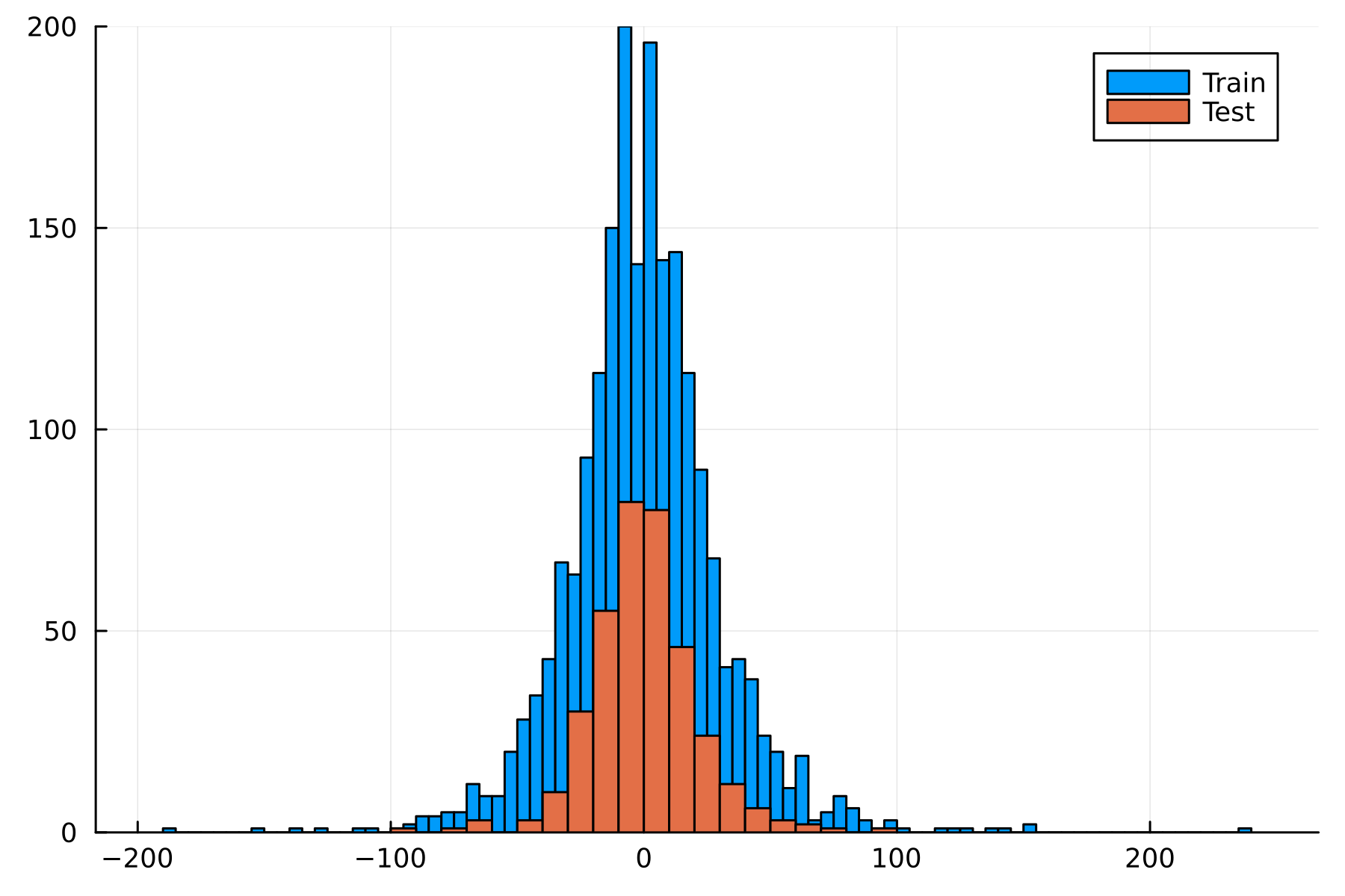
Like I said, it’s a quirk of the dataset, but something to bear in mind for the rest of the examples.
Let’s look at the predicted values of this first neural net and how they line up with reality. Plus, we can compare it to the linear model. For the linear model, you just need to run predict and pass in the test dataset. Similarly, with the neural net, we evaluate the trained model on the testing matrix.
nnTest = DataFrame(t=tsTest, delta_vNorm_nn = vec(flux_model(xTest)'))
spyTest.delta_vNorm_lin = predict(linearModel, spyTest)
spyTest = leftjoin(spyTest, nnTest, on = :t);
As we are predicting the change in the daily volume, we need to add back in the previous value to get our predicted daily volume.
spyTest = @transform(spyTest, :v_nn = :prev_vNorm .+ :delta_vNorm_nn, :v_lin = :prev_vNorm + :delta_vNorm_lin);
sort!(spyTest, :t);
And then plotting
p = plot(spyTest.t, spyTest.vNorm, label = "True",  dpi=300, background_color = :transparent)
p = plot!(p, spyTest.t, spyTest.v_nn, label = "NN")
p = plot!(p, spyTest.t, spyTest.v_lin, label = "Linear")
p
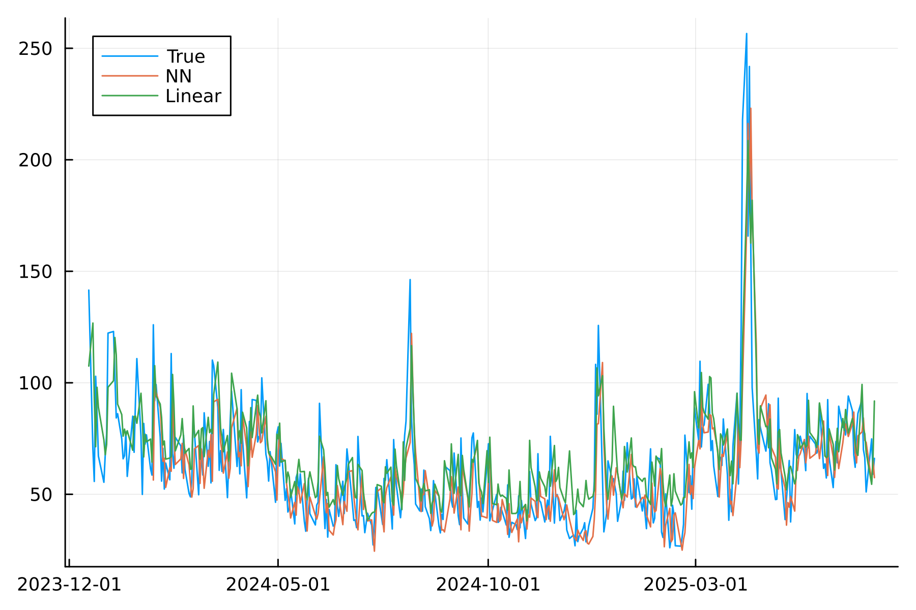
Things line up quite well, nothing outrageous.
In terms of performance, we calculate the MSE from the dataframe.
@combine(dropmissing(spyTest),
          :NN = mean((:vNorm .- :v_nn).^2),
          :Lin = mean((:vNorm .- :v_lin).^2))
| NN | Lin |
|---|---|
| 405.55 | 370.57 |
The linear model is doing better so far.
2 Layer Neural Nets
We are now in the realm of multi-layer perceptrons (MLPs) and have introduced many more parameters into the model. We can also now build more complicated interactions with each layer.
In Flux, building out more layers is simple; you are chaining different dense layers together. We are choosing to have a fully connected MLP with 2 layers, with all the variables passed through.
flux_model2 = Flux.Chain(Dense(size(x, 1), size(x, 1)), Dense(size(x, 1), 1))

flux_model2, allTrainLoss, allTestLoss = train((xTrain, yTrain), (xTest, yTest), flux_model2, flux_loss; epochs = 1000, eta = 1e-6);
This trains in the same amount of time with the same train/test loss pattern. Again, assessing the MSE of this bigger model.
nnhTest = DataFrame(t=tsTest, delta_vNorm_nnh = vec(flux_model2(xTest)'))
spyTest = leftjoin(spyTest, nnhTest, on = :t);

spyTest = @transform(spyTest, :v_nnh = :prev_vNorm .+ :delta_vNorm_nnh)
@combine(dropmissing(spyTest), :NN = mean((:vNorm .- :v_nn).^2),
                               :Lin = mean((:vNorm .- :v_lin).^2),
                               :NNH = mean((:vNorm .- :v_nnh).^2))
| NN | Lin | NNH |
|---|---|---|
| 405.55 | 370.57 | 401.424 |
This has improved on the 1-layer neural net, but still no better than the linear model.
Neural Net Regularisation
The linear model has 13 parameters, the 1-layer neural net has 42 parameters, and the 2-layer net has 1,764 parameters. This is a rapid growth in complexity which raises the likelihood that the model starts to overfit. How do we make sure the neural net models only pick out the key parameters and regularise themselves?
We have two options: add a penalisation score in the loss function that bounds the total size of the coefficients or introduce something called a dropout layer.
Penalising the Loss Function
You can extend regularisation into neural networks the same way you do linear models. You add an additional term to the loss function that penalises the total combined size of the coefficients.
function flux_loss_reg(flux_model, x, y)
    flux_loss(flux_model, x, y) + sum(x->sum(abs2, x), Flux.trainables(flux_model))
end
Therefore, if the model wants to allocate more weight to 1 parameter, it needs to take some weight from another. This acts as a balancing mechanism and should reduce the chance of overfitting.
We use this new loss function with the 2-layer net.
flux_model = Flux.Chain(Dense(size(x, 1), size(x, 1)), Dense(size(x, 1), 1))
flux_model, allTrainLoss, allTestLoss = train((xTrain, yTrain), (xTest, yTest), flux_model, flux_loss_reg; epochs = 1000, eta = 1e-6);
| NN | Lin | NNH | NNHR |
|---|---|---|---|
| 405.55 | 370.57 | 401.424 | 388.548 |
So slightly better than the unregularised version.
Neural Net Dropout Layers
An alternative way of regularising a network is to introduce a dropout layer. Dropout randomly sets the output of a node to zero during the training phase, which means the net has fewer parameters to optimise over and reduces the possibility of overfitting. When it comes to inference, all of the nodes are included but rescaled by the dropout probability. The original dropout paper is an engaging read - Dropout: A Simple Way to Prevent Neural Networks from Overfitting.
Again, very simple to use dropout in Julia and Flux; it is just another type of layer.
flux_model3 = Flux.Chain(Dense(size(x, 1), size(x, 1)), Dropout(0.5), Dense(size(x, 1), 1))

flux_model3, allTrainLoss, allTestLoss = train((xTrain, yTrain), (xTest, yTest), flux_model3, flux_loss; epochs = 250, eta = 1e-6);
For the final time, let’s evaluate this model on the test set and calculate the MSE.
nndTest = DataFrame(t=tsTest, delta_vNorm_nnd = vec(flux_model3(xTest)'))
spyTest = leftjoin(spyTest, nndTest, on = :t);

spyTest = @transform(spyTest, :v_nnd = :prev_vNorm .+ :delta_vNorm_nnd)
@combine(dropmissing(spyTest), :NN = mean((:vNorm .- :v_nn).^2),
                               :Lin = mean((:vNorm .- :v_lin).^2),
                               :NNH = mean((:vNorm .- :v_nnh).^2),
                               :NND = mean((:vNorm .- :v_nnd).^2))
| NN | Lin | NNH | NNHR | NNHD |
|---|---|---|---|---|
| 405.55 | 370.57 | 401.424 | 388.548 | 411.105 |
The worst model so far!
Conclusion
So the linear model is still winning. The neural net and various iterations haven’t improved on this simple model, and the best neural net was the 2-layer with regularisation.
It must be noted that this problem isn’t exactly hard, and the amount of data is relatively small, so it is unsurprising that the added complexity of the neural nets hasn’t added anything. It’s hardly a ‘deep learning’ problem!
I’ve also not gone crazy with the neural net optimisations. You can include more layers, change the number of nodes in the layers, change the activation functions, and change the loss function - all sorts of things that could be tweaked and improve the model.
Hopefully I’ve not just added to the slop of neural net finance tutorials and you’ve found something useful. Unfortunately, the neural nets haven’t beaten the linear model, which shows you can’t just jump into the fancy tools without looking at the simpler models.
Other Julia/Finance Posts
For more quant finance tutorials check out some of my older posts.