A Fundamental FX Factor Model
I’ve been reading The Elements of Quantitative Investing to branch out from my usual high-frequency finance to something slower or mid-frequency. Factor models are a big part of this quant topic, and I’m trying to get a deeper understanding by following the book and applying the process to FX data.
Enjoy these types of posts? Then sign up for my newsletter.
Factor models provide a mechanism for explaining returns. They are multivariate models that break down the features that drive an asset’s performance. The key assumption is that each individual asset’s return is not independent of the others, but there are common factors that drive returns and an asset’s sensitivity to those factors drives its returns. In equities, you’ll hear of value and momentum factors, and there are even ETFs that you can invest in for exposure to those factors. We want to come up with something similar in the FX space.
A factor model attempts to explain asset-universe return behaviour. From this you can start to build portfolios, decompose risk across the different factors, and even look at returns not explained by the factors, which in turn becomes alpha research. These types of models are the foundation of many other quant topics, so it’s good to get a handle on them.
I will start by getting the data and the features into place. Part of that is using the DXY functions from my previous post (Making Sense of the DXY) and adding some new ETF data. I’ll then run two models: one to explain price moves over time and another to explain price moves between currencies themselves. Using the models in tandem forms the FX factor model. We will then explore the specific factors and how you can build factor portfolios from different currency pairs.
FX vs Equities
Typically, factor models and most academic research in this field use equity data. However, I am an FX man at heart (for my sins?) and so I want to use currency data. This restricts the universe to about 30 assets rather than the 2,000 US stocks. Therefore, to overcome the small sample size, we will use weekly data rather than monthly.
Monthly data will remove as much “trading” noise as possible. You want the price moves to reflect the underlying performance of the asset and not the day-to-day flows and execution noise. Daily data isn’t an option as FX trades 24 hours a day but the ETFs only trade during the regular market hours. This presents a synchronisation problem. A currency move could happen overnight based on some headlines hours before the ETF is even open for trading. So we will split the difference and use weekly data. This should give us enough data while keeping the overall price movements based on the same time period and information.
Another problem with FX data is a lack of descriptive features. Again, in equities, you have the financial reports of a company, things like price to book and market capitilisation but these have no equivalent in FX so we need to a different way of coming up with characteristics. For this I’ll be using ETFs to try and see what macro features might move the currency pairs.
The Data Pipeline
We are bringing together ETF, currency, and DXY data. This is all simple to pull from twelvedata.
Downloading and Preparing the ETF Data
I’ll be using different macro ETFs as general factors. These four ETFs proxy the major macro drivers:
- VTI (Risk Appetite): When stocks rally, investors move from cash to risk assets, weakening the dollar (capital flows out of US). When stocks fall, the reverse.
- BND (Interest Rates): Bond prices move inversely to rates. Rising US rates strengthen the dollar; falling rates weaken it.
- GLD (Inflation/Uncertainty): Gold rallies when inflation forecasts rise or geopolitical risk spikes, often correlated with currency volatility.
- USO (Commodity Risk): Oil is priced in dollars. Oil rallies often reflect emerging market demand, shifting currency flows.
Each of these ETFs forms a standard macro-economic indicator that I suspect currencies might respond to. You could go further and break down the stocks into different regions or sizes (small-cap, large-cap etc.) and likewise for the bonds, which could be broken down by country. But for now, these are a good high-level weather vane for how the global economy is moving.
We will be using the same functions from my previous post, just updating it to save at a weekly frequency. Then we load those files, combine everything, and calculate the log returns.
etfs = ["GLD", "BND", "VTI", "USO"]
etfDF = [load_data(etf) for etf in etfs]
etfDF = pl.concat(etfDF)
etfDF = etfDF.sort("datetime")

etfDF = etfDF.with_columns(
    pl.col("close").log().diff().over("ccy").alias("log_return"))
We need to normalise the log returns by rolling volatility. To calculate the volatility, we take the standard deviation of the returns in a 52-week period.
etfDF = etfDF.with_columns(pl.col("log_return").rolling_std(window_size=52).over("ccy").alias("vol_52"))
etfDF = etfDF.with_columns((pl.col("log_return")/pl.col("vol_52")).alias("log_return_scaled"))


etfDF = etfDF.select(pl.col("datetime"), pl.col("ccy"), pl.col("log_return_scaled"))
etfDF = etfDF.pivot(values="log_return_scaled", index="datetime", columns="ccy")
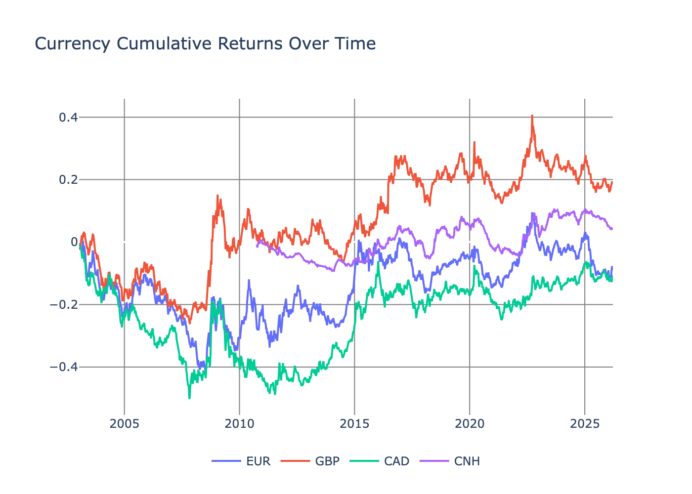
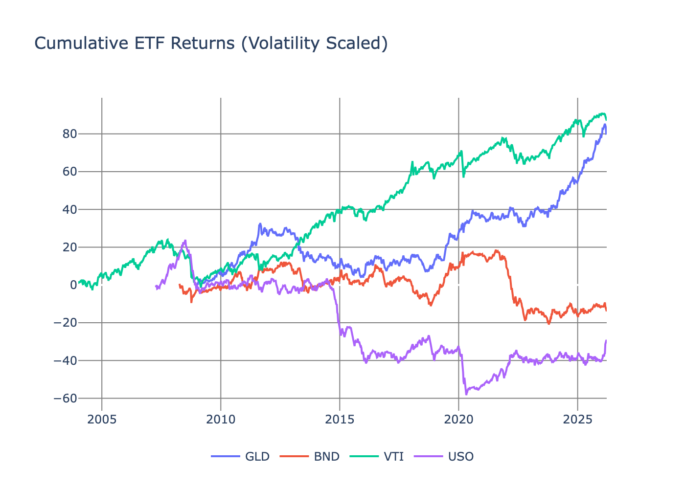
When we plot these normalised ETF returns, they line up with what we expect.
We need to ensure the different ETFs aren’t overly correlated. Highly correlated ETF returns would indicate redundant information, and multicollinearity in our regression analysis would lead to unstable coefficient estimates. Ideally, the ETF returns should capture distinct dimensions of macro risk.
Polars makes it easy to calculate the correlations over time with the rolling_corr function.
etfDFCorr = etfDF.with_columns(
    pl.rolling_corr("VTI", "USO", window_size=52).alias("VTI_USO_corr"),
    pl.rolling_corr("VTI", "BND", window_size=52).alias("VTI_BND_corr"),
    pl.rolling_corr("VTI", "GLD", window_size=52).alias("VTI_GLD_corr"),
    pl.rolling_corr("USO", "GLD", window_size=52).alias("USO_GLD_corr")
    ).drop_nulls()
Plotting these correlations gives us confidence that everything is reasonable.
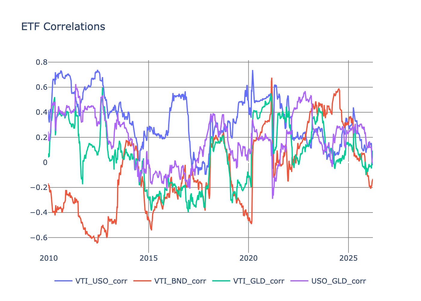
At worst, we see a 0.6 correlation, which is just about acceptable as it only occurs for a brief period.
Sidenote: it’s interesting how stock–bond correlation hasn’t been negative since 2020. Thinking out loud, but that must have some big consequences for the risk profile of the 60/40 allocation. Another post for another day prehaps.
Now, onto the FX data.
Getting the FX + DXY Data
Again, following my last post I’m now just pulling the weekly data instead of daily. I’ve also wrapped the DXY calculations from my previous post (Making Sense of the DXY) into a nice function.
We load across the 33 currencies available.
dfs = [load_data(ccy) for ccy in ccys]
df = pl.concat(dfs)
df = df.sort("datetime")
df = df.drop("open", "high", "low")
Then join the DXY and ETF data.
dxy = load_dxy()
df = df.join(dxy.select(pl.col("datetime"), pl.col("dxy_close")), on="datetime", how="left")
df = df.join(etfDF, on="datetime", how="left")
We then calculate the returns and the 1-month, 6-month and 1-year momentum factors.
df = df.with_columns(
    pl.col("close").log().diff().over("ccy").alias("log_return"),
    pl.col("dxy_close").log().diff().over("ccy").alias("dxy_log_return"),
    pl.col("close").log().diff(n=4).shift(1).over("ccy").alias("log_return_4"),
    pl.col("close").log().diff(n=26).shift(1).over("ccy").alias("log_return_26"),
    pl.col("close").log().diff(n=52).shift(1).over("ccy").alias("log_return_52")
)
Like the ETF returns we also want to normalise the currency returns and DXY returns by their rolling volatility.
df = df.with_columns(pl.col("log_return").rolling_std(window_size=52).over("ccy").alias("vol_52"))
df = df.with_columns((pl.col("log_return")/pl.col("vol_52")).alias("log_return_scaled"))

df = df.with_columns(pl.col("dxy_log_return").rolling_std(window_size=52).over("ccy").alias("dxy_vol_52"))
df = df.with_columns((pl.col("dxy_log_return")/pl.col("dxy_vol_52")).alias("dxy_log_return_scaled"))
We normalise the momentum features in the same way.
df = df.with_columns((pl.col("log_return_4")/pl.col("log_return_4_vol_52")).alias("log_return_4_scaled"))
df = df.with_columns((pl.col("log_return_26")/pl.col("log_return_26_vol_52")).alias("log_return_26_scaled"))
df = df.with_columns((pl.col("log_return_52")/pl.col("log_return_52_vol_52")).alias("log_return_52_scaled"))
It is also recommended you winsorise the return data. This involves replacing the extreme values with the 5% quantiles and a simple polars function. This reduces the influence of outliers in the models and just keeps the data a bit cleaner.
cols = ["log_return_scaled", "dxy_log_return_scaled", "log_return_4_scaled", "log_return_26_scaled", "log_return_52_scaled",
       "GLD", "BND", "VTI", "USO"]

df = df.with_columns([
    pl.col(c).clip(
        pl.col(c).quantile(0.05),
        pl.col(c).quantile(0.95)
    ).alias(f"{c}_clipped")
    for c in cols
])
With the data collected we can now move on to some modelling.
FX Return Characteristics
We need to build a dataset of characteristics per currency pair. These are potential features that will explain an individual currency’s return over time.
Mathematically
\[R = \beta X,\]where \(R\) is the currency return, \(X\) are the returns from other assets and we want to estimate \(\beta\). If a currency is sensitive to oil, then it will have some element of dependence on the oil ETF USO and \(\beta _\text{USO}\) will capture that effect.
\(X\) contains the weekly values of
- Weekly DXY return
- Global stocks (VTI)
- Global bonds (AGG)
- Oil (USO)
- Gold (GLD)
- The currency’s momentum at 1, 6 and 12 month intervals.
The model is fitted per currency individually as a rolling one-year regression. We use volatility-normalised returns so the \(\beta\)s are more stable over time.
import statsmodels.formula.api as smf
from statsmodels.regression.rolling import RollingOLS

allParams = []
# sort the subdata by datetime to ensure the rolling regression works correctly
for ccy in ccys:
    subDF = df.filter(pl.col("ccy") == ccy).drop_nulls().sort("datetime")
    mod = RollingOLS.from_formula("log_return_scaled_clipped ~ dxy_log_return_scaled_clipped + GLD_clipped + BND_clipped + VTI_clipped + USO_clipped + log_return_4_scaled_clipped + log_return_26_scaled_clipped + log_return_52_scaled_clipped",
                window = 52,
                data=subDF).fit()

    paramDF = pl.from_pandas(mod.params)
    paramDF = paramDF.with_columns(ccy=pl.lit(ccy),
                                   datetime = subDF["datetime"],
                                   log_return = subDF["log_return"],
                                   log_return_prev = subDF["log_return"].shift(1),
                                   r2 = mod.rsquared_adj.values,
                                   vol_52 = subDF["vol_52"])

    allParams.append(paramDF)


allParams = pl.concat(allParams).drop_nulls().sort("datetime")
We save the \(\beta\) time series, the \(R^2\) values, and the volatility.
To make sure the regression is doing a good job for all the time periods we plot the \(R^2\) for a few currencies.
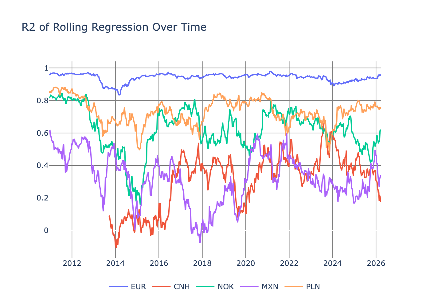
They are all the right order of magnitude with CNH and MXN being the worst but still manageable.
If we average over currency pairs and time, we get a rough understanding of the \(\beta\) values.
betaSummary = (
    allParams
    .unpivot(index=["datetime", "ccy"])
    .group_by("variable")
    .agg(
        pl.col("value").mean().alias("mean"),
        pl.col("value").std().alias("std"),
        pl.col("value").min().alias("min"),
        pl.col("value").max().alias("max")
    )
    .sort("mean", descending=True)
)
betaSummary.filter(pl.col("variable").str.contains("dxy_log_return|log_return_4|log_return_26|log_return_52|VTI|BND|GLD|USO|Intercept"))
| Variable | Mean | Std | Min | Max |
|---|---|---|---|---|
| dxy_log_return_scaled | 0.485 | 0.327 | -0.452 | 1.34 |
| Intercept | 0.0853 | 0.385 | -2.26 | 25.1 |
| USO | -0.0222 | 0.166 | -0.942 | 0.730 |
| BND | -0.0267 | 0.176 | -0.970 | 0.788 |
| log_return_4_scaled | -0.0341 | 0.146 | -0.864 | 1.69 |
| log_return_52_scaled | -0.0525 | 0.192 | -1.92 | 0.932 |
| log_return_26_scaled | -0.0591 | 0.180 | -1.50 | 0.895 |
| GLD | -0.0636 | 0.179 | -1.06 | 0.599 |
| VTI | -0.149 | 0.206 | -0.982 | 0.844 |
DXY is the main driver, with a negative dependence on VTI. This makes sense and lines up with our beliefs: if stocks are doing badly, it’s likely people sold them for cash, and likewise when stocks are doing well people are moving from cash into equities. This helps confirm VTI as a general risk-on/risk-off factor.
It’s frustrating that the intercept has a large average \(\beta\) value, as it means we are missing drivers of currency returns. An obvious omission is the carry factor and how interest rates across countries drive currency returns. Annoyingly, it’s hard to get free data for that, so we will have to make do for now.
We’ve now got a picture of how much each currency depends on macro factors but this tells us about individual currencies in isolation. We now need to know if differences in these sensitivities explain why some pairs outperform others.
To answer that, we regress across currency pairs at each point in time. This is known as cross sectional regression.
Cross Sectional Regression for Currency Returns
From the first regression we have currency characteristics over time. For the cross-sectional regression, we now use all the currencies per week and then run the regression to see if the sensitivity to the factors (the \(\beta\)s) explains the returns.
We also add in a currency group factor as an additional characteristic that classifies broad groups of currency pairs.
allParams = allParams.with_columns(
    pl.col("ccy").map_elements(ccy_group_map).alias("ccyGroup")
    )
We normalise the \(\beta\)’s across the currency pairs which helps keep everything comparable.
This time mathematically,
\[R = \lambda B,\]where \(R\) are the currency returns for a given week and \(B\) is the matrix of normalised \(\beta\) values and the currency group indicator. We are using simple weighted regression to estimate \(\lambda\). The weights use the inverse of the volatility to reduce the impact of high volatility pairs.
allParams2 = []

factor_cols = ["dxy_log_return_scaled_clipped", "GLD_clipped", "BND_clipped", "VTI_clipped", "USO_clipped", "log_return_4_scaled_clipped", "log_return_26_scaled_clipped", "log_return_52_scaled_clipped"]

for (i, dt) in enumerate(allParams["datetime"].unique()):
    subDF = allParams.filter(pl.col("datetime") == dt)

    subDF = subDF.with_columns([
    ((pl.col(c) - pl.col(c).mean().over("datetime")) /
      pl.col(c).std().over("datetime")).alias(f"{c}_scaled")
    for c in factor_cols
    ])

    csr = smf.wls("log_return_prev ~ ccyGroup + dxy_log_return_scaled_clipped_scaled + GLD_clipped_scaled + BND_clipped_scaled + VTI_clipped_scaled + USO_clipped_scaled + log_return_4_scaled_clipped_scaled + log_return_26_scaled_clipped_scaled + log_return_52_scaled_clipped_scaled",
                  data=subDF, weights=1/(subDF["vol_52"]**2)).fit()

    paramsRes = pl.DataFrame(data = [[x] for x in csr.params.values],
             schema=list(csr.params.index.values))

    paramsRes = paramsRes.with_columns(datetime=pl.lit(dt))
    allParams2.append(paramsRes)

allParams2 = pl.concat(allParams2).drop_nulls().sort("datetime")
allParams2 = allParams2.filter(pl.col("datetime") != pl.date(2009,4, 14))
allParams2 = allParams2.filter(pl.col("datetime") != pl.date(2009,4, 15))
allParams2 = allParams2.filter(pl.col("datetime") != pl.date(2009,4, 16))
To check the performance of the regression, we plot the \(R^2\) over time.
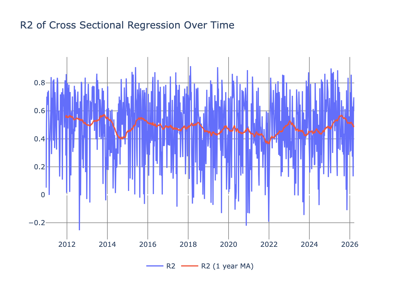
Again noisy, but the rolling average moves around 0.4, which is a respectable value.
We then calculate the t-stats by taking the average fitted parameters and dividing by the standard error.
| variable | avg | std | N | std_error | t_stat |
|---|---|---|---|---|---|
| ccyGroup[T.EM] | 0.00113 | 0.00920 | 797 | 0.000326 | 3.46 |
| log_return_4_scaled_clipped_scaled | 0.000266 | 0.00240 | 797 | 0.000085 | 3.13 |
| log_return_26_scaled_clipped_scaled | 0.000324 | 0.00295 | 797 | 0.000105 | 3.10 |
| ccyGroup[T.SCANDI] | 0.000586 | 0.00982 | 797 | 0.000348 | 1.68 |
| ccyGroup[T.G7] | 0.000452 | 0.00776 | 797 | 0.000275 | 1.64 |
| ccyGroup[T.CEMA] | 0.000584 | 0.0101 | 797 | 0.000358 | 1.63 |
| log_return_52_scaled_clipped_scaled | 0.000135 | 0.00291 | 797 | 0.000103 | 1.31 |
| ccyGroup[T.LATAM] | 0.000404 | 0.00949 | 797 | 0.000336 | 1.20 |
| VTI_clipped_scaled | 0.000102 | 0.00319 | 797 | 0.000113 | 0.906 |
| GLD_clipped_scaled | 0.0000670 | 0.00284 | 797 | 0.000101 | 0.668 |
| Intercept | 0.0000620 | 0.00520 | 797 | 0.000184 | 0.335 |
| USO_clipped_scaled | -0.00000200 | 0.00285 | 797 | 0.000101 | -0.0175 |
| BND_clipped_scaled | -0.0000840 | 0.00289 | 797 | 0.000102 | -0.822 |
| dxy_log_return_scaled_clipped_scaled | -0.000340 | 0.00398 | 797 | 0.000141 | -2.42 |
Anything over 2 is deemed significant, which gives us:
- EM pairs
- 1-month momentum
- 6-month momentum
- DXY return
We can look at the returns of these factors (just the significant ones).
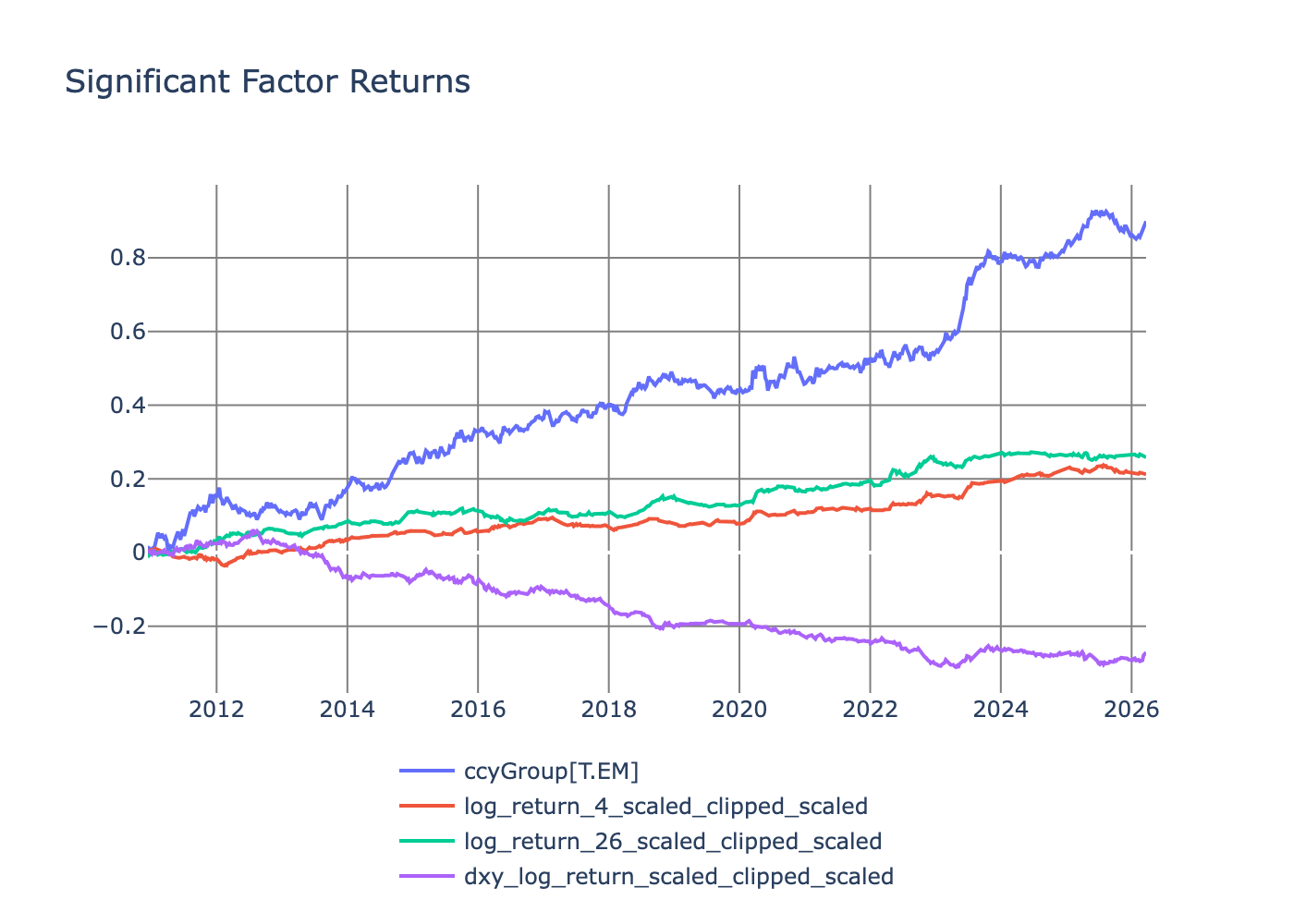
The EM factor has the best return, and all the factor returns are positive except the DXY factor. For the EM factor, the coefficients are significant and positive; therefore we interpret this as investors demanding a premium return for holding EM pairs — at least the ones I’ve tagged as EM. Similarly, the two momentum factors command a similar premium.
But what currency pairs do you need to buy and sell to get these factor returns?
How to Build the Factor Portfolios
After fitting the cross sectional regression model we arrive at \(\hat{\lambda}\) which are the the factor returns. What we now want are the currency weights that will get us to the factor returns
\[\hat{\lambda} = w R,\]after some maths you arrive at
\[w = (B^TB)^{−1}B^T.\]Easy enough to translate into Python.
ccyWeights = []

for dt in allParams["datetime"].unique():
    betas = allParams.select(pl.exclude("log_return", "log_return_prev", "ccyGroup", "r2", "vol_52"))
    betas = betas.filter(pl.col("datetime") == dt)
    B = betas.select(pl.exclude("datetime", "ccy")).to_numpy()

    W = np.linalg.solve(B.T @ B, B.T)

    res = pl.DataFrame(W, schema=betas["ccy"].to_list()).with_columns(
        pl.Series(name="factor", values=betas.select(pl.exclude("datetime", "ccy")).columns),
        datetime = betas["datetime"][0]
        ).unpivot(index=["datetime","factor"])

    ccyWeights.append(res)

ccyWeights = pl.concat(ccyWeights)
As we are using the \(\beta\) matrix, we get a time series of weights. The currencies’ underlying sensitivities to the different features change over time, meaning that they will undergo different weighting in the factor portfolios over time too.
After running that calculation we get to the currency rates.
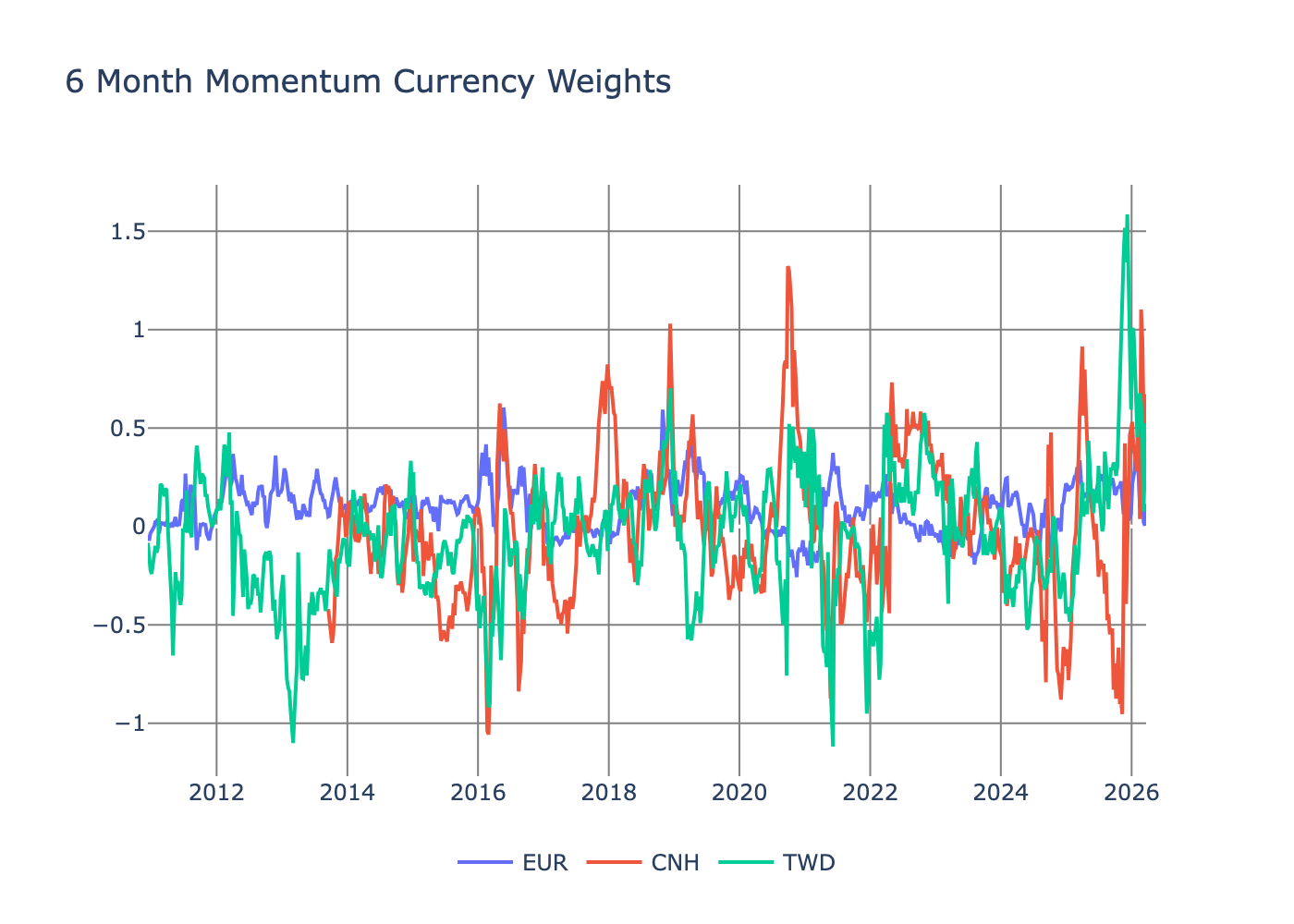
For the momentum factor, EUR hugs zero more than the other selected currencies.
If we look at the DXY factor and the currency weights for 2026 to have a more realistic view of how they are changing, we can see much more stability.
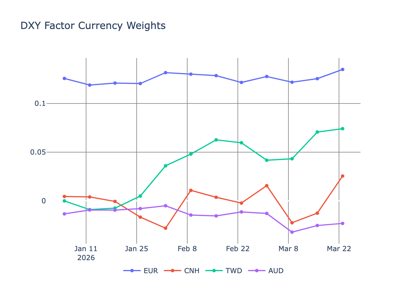
Small changes around EUR; CNH has hovered around zero; TWD has gone long since February; and AUD has picked up a short position. Given these are weekly weights, it’s good that there aren’t any wild swings, since big changes in positioning would lead to larger transaction costs.
Conclusion
Done. We’ve built a fundamental FX factor model. It’s involved, with lots of different ways to fall over, but we made it. Four factors were significant: 1-month momentum, 6-month momentum, DXY, and the EM factor. The smaller size of the FX universe compared to equities means there is less data through time and across assets. Also, the underlying \(\beta\)s are noisy given the tighter return ranges compared to equities. There is also a case that regime changes average things out to zero, but it’s hard to see that in the data. However, this model can help in hedging and explaining risk, but not serve as a source of expected returns.
If you’ve looked at FX factor models before, you’ll realise I’ve missed a pretty significant factor — carry. It’s very hard to get free data to calculate the carry factor across the full universe of currencies. I’m saving it for another day for a smaller set of pairs where there is data.
So I hope this has been a good walkthrough and explainer on how to approach these factor models.