Making Sense of the DXY
My day job is in quant trading, but there’s another fascinating world: quantitative investing. While I focus on latencies and execution, quant investors are busy building the most efficient portfolios and ensuring they extract pure alpha. Not one to stay in my lane, I’m using this blog post as an opportunity to dive into the world of quant investing and level up my knowledge.
Enjoy these types of posts? Then sign up for my newsletter.
Now most quant investing examples use equities as the underlying asset class, but I am an FX man, so will be replacing Apple and Microsoft with Euro’s and Yen. In some ways, this is easier; I just have to worry about 30-odd currencies as my investible universe compared to the thousands, if not hundreds of thousands, of different stocks. But in many ways it’s harder. What drives FX returns is at a much higher macro-level compared to an individual stock, and things like central banks changing interest rates, government policy changes are difficult to translate to a dataset compared to the price-to-book ratio of a stock. Still, we will give it a go.
In short, we want to better understand what can influence a currency’s return and produce a systematic model. This post is going to start with the basics, pulling in the right data, building a proxy to the overall FX market and ending with some basic regressions.
Twelve Data
For any quant investing model, we need to start with data. I’m always on the hunt for new sources, and twelvedata is the latest one to come across my radar. It has a generous free tier and, more importantly, has FX data across all the main pairs. Plus, it has a Python API that is dead simple to use. This makes it ideal for this string of posts.
Sign up and get your API key, and you can follow along.
from twelvedata import TDClient

td = TDClient(apikey=API_KEY)

td.time_series(
        symbol="USD/JPY",
        interval="1day",
        start_date="2025-01-01",
        end_date="2026-03-01",
        outputsize=5000).as_json()
This returns the daily timeseries of USDJPY since 2025 til March 2026, formatted as a JSON. Pretty simple to then go from that to a dataframe or however you want to deal with the data.
I don’t want to get blocked by the API limits, so I’m going to save the JSON objects locally.
def download_data(td, ccy, start_date, end_date):
    return td.time_series(
        symbol=f"USD/{ccy}",
        interval="1day",
        start_date=start_date,
        end_date=end_date,
        outputsize=5000
    )

def save_data(data, ccy):
    with open(f"data/{ccy}.json", "w") as f:
        json.dump(data.as_json(), f)

def download_and_save_data(td, ccy, start_date, end_date):
    file_path = f"data/{ccy}.json"
    if os.path.exists(file_path):
        print(f"File for {ccy} already exists. Skipping download.")
        return False
    print(f"Downloading data for {ccy}...")
    data = download_data(td, ccy, start_date, end_date)
    print(f"Saving data for {ccy}...")
    save_data(data, ccy)
    print(f"Data for {ccy} downloaded and saved successfully.")
    print("Sleeping for 8 seconds to avoid hitting API rate limits...")
    time.sleep(8)
    return True
Then, to load the data for a particular currency, we have a separate function.
def load_data(ccy):
    df = pl.read_json(f'data/{ccy}.json')
    df = df.with_columns(
        pl.col("datetime").cast(pl.Date),
        ccy=pl.lit(ccy),
        open=pl.col("open").cast(pl.Float64),
        high=pl.col("high").cast(pl.Float64),
        low=pl.col("low").cast(pl.Float64),
        close=pl.col("close").cast(pl.Float64))
    return df
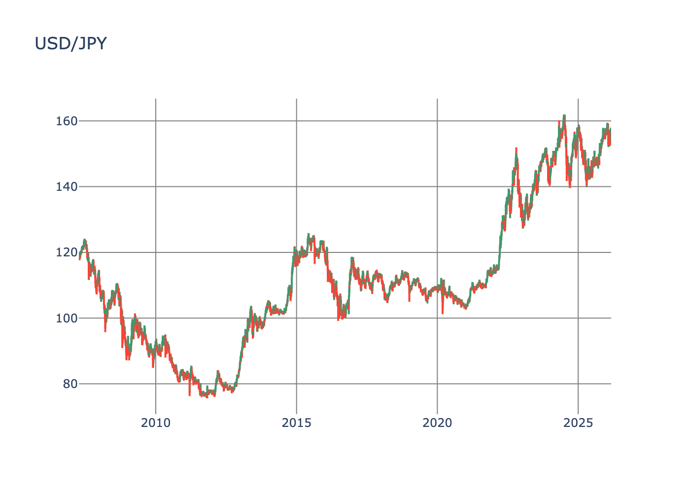
To make sure everything is working nicely, let’s load and plot JPY.
df = load_data("JPY")

fig = go.Figure(data=go.Ohlc(x=df['datetime'],
                    open=df['open'],
                    high=df['high'],
                    low=df['low'],
                    close=df['close']))

fig.show()
All looks good, so now we can download whatever pair our heart desires. Which leads us to the next part.
What is the DXY?
In my mind, the DXY is the FX equivalent of the S&P500. It gives a general indication of how the dollar’s value is changing by using the exchange rate of EUR, JPY, CHF, GBP, CAD and SEK vs the dollar. It’s calculated as a geometric weighted average of these six currencies, and given the dollar’s dominance in the FX market, it works as a reasonable proxy of how the overall FX market is moving.
If we cast our mind back to the Capital Asset Pricing Model, an asset’s expected return can be broken down to its \(\alpha\) active return and its sensitivity to the market, \(r_m\). The strength of this sensitivity is \(\beta\).
\[r_i = \alpha_i + \beta_i r_m\]In equities, \(r_i\) is a single stock and \(r_m\) is some measure of the overall market return (S&P500, FTSE100, etc.). In FX, \(r_i\) is an individual currency and \(r_m\) is the DXY. This gives us an easy quantitative model to judge how a currency’s return is driven by the overall movement in the dollar.
Now you can either read the DXY from a market data source (expensive) or you can calculate it yourself.
Calculating the DXY
The formula for the DXY is in a pdf here: U.S. Dollar Index Contracts. It’s a simple weighted geometric average, so we just need the individual currency prices, and we can implement the calculation.
dfs = [load_data(ccy) for ccy in ["EUR", "JPY", "GBP", "CAD", "SEK", "CHF"]]
combined_df = pl.concat(dfs)
combined_df = combined_df.sort("datetime")
The more eagle-eyed readers might have noticed that I’m saving down some of the pairs the ‘wrong’ way round. USDEUR instead of EURUSD, USDGBP instead of GBPUSD, etc. This is because the DXY needs to flip everything into USD base terms, so in the weighting, some of the negatives are changed to positive.
dxyWeightings = {
    "EUR": 0.576,
    "JPY": 0.136,
    "GBP": 0.119,
    "CAD": 0.091,
    "SEK": 0.042,
    "CHF": 0.036,
    "const": 50.14348112}

weights_df = pl.DataFrame(list(dxyWeightings.items()), schema=["ccy","weight"])
combined_df = combined_df.join(weights_df, on="ccy", how="left")
So now we have a dataframe of the relevant prices joined by the weightings.
Step 1: exponentiate the 4 prices by the right power.
combined_df = combined_df.with_columns(
    (pl.col("open") ** pl.col("weight")).alias("open_weighted"),
    (pl.col("high") ** pl.col("weight")).alias("high_weighted"),
    (pl.col("low") ** pl.col("weight")).alias("low_weighted"),
    (pl.col("close") ** pl.col("weight")).alias("close_weighted")
Step 2: For each day, take the product and multiply it by the constant.
dxy = combined_df.group_by("datetime").agg(
    pl.col("open_weighted").product().alias("dxy_open"),
    pl.col("high_weighted").product().alias("dxy_high"),
    pl.col("low_weighted").product().alias("dxy_low"),
    pl.col("close_weighted").product().alias("dxy_close")
).with_columns(
    pl.col('dxy_open')*dxyWeightings["const"],
    pl.col('dxy_high')*dxyWeightings["const"],
    pl.col('dxy_low')*dxyWeightings["const"],
    pl.col('dxy_close')*dxyWeightings["const"])
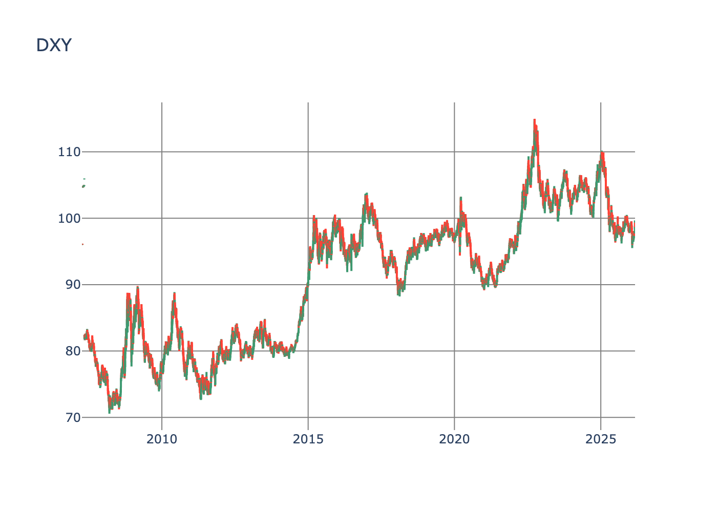
[Alt text: Line chart depicting daily DXY values. The x-axis shows time, and the y-axis shows the DXY value. The chart provides a clear view of the daily movement of the DXY.]
If you compare it to the Yahoo Finance DXY plot, it looks pretty similar, so I’m pretty confident this is all correct.
Individual Currency \(\beta\)’s
Now we can go on to measuring the currencies \(\beta\) values. This is a simple linear regression of the log returns of an individual currency vs the log returns of the DXY.
We need to load in more currency pairs.
dfs = [load_data(ccy) for ccy in all_pairs]
combined_df = pl.concat(dfs)
combined_df = combined_df.sort("datetime")
For the regression, we need the individual currency returns and also the DXY returns. Simple log return calculation, and then join the DXY frame onto the individual currencies.
combined_df = combined_df.with_columns(
    pl.col("close").log().diff().over("ccy").alias("log_return")
)

dxy = dxy.with_columns(
    pl.col("dxy_close").log().diff().alias("dxy_log_return")
)

combined_df = combined_df.join(dxy, on="datetime", how="left")
We will do a rolling regression using a 252-day look back, which is roughly the number of trading days in a year.
from statsmodels.regression.rolling import RollingOLS

allParams = []

for ccy in ["EUR", "SEK", "CNH", "TWD", "TRY"]:

    subDF = combined_df.filter(pl.col("ccy") == ccy)
    mod = RollingOLS.from_formula("log_return ~ dxy_log_return", data=subDF, window=252)
    rres = mod.fit()

    paramDF = pl.from_pandas(rres.params)
    paramDF = paramDF.with_columns(ccy=pl.lit(ccy), Date = subDF["datetime"])
    allParams.append(paramDF)

allParams = pl.concat(allParams)
To examine the results, we plot the \(\beta_i\) value over time for some different currencies.

EUR (green) is close to 1, which aligns with intuition as it’s the largest weight of the DXY calculation. TRY has the lowest \(\beta\) out of these pairs, which suggests its returns are not driven by the overall dollar returns, again, makes sense given TRY’s movements reflect the underlying macroeconomics of TRY. SEK has a consistent \(\beta > 1\) which again suggests it’s very susceptible to general dollar moves. It’s not pictured, but HKD comes out with the lowest \(\beta\), which is reassuring as it is pegged to the dollar.
Overall, do these \(\beta\)’s tell us much? Not really, but it is interesting to measure, and this is the foundation needed before we start looking at other factors that might influence the daily currency movements. These can be things like momentum, oil/gold sensitivity, etc.
Conclusion
From this, we have built up a new dataset of daily currency prices and now have daily DXY values too. This has given the underpinnings of an FX factor model, and next time we can start looking at other components that could explain currency movements.
Loosely related is my post on Currency Hedging and Principal Component Analysis and Dipping My Toes into ETF Correlations.