A Statistical FX Factor Model
Factor models attempt to explain asset returns. You can approach this in two ways: define the factors you think are relevant, or use statistical learning to build the relevant factors from the data. My previous post took the first approach. This post will use principal component analysis (PCA) to let the data tell us which factors are most relevant in an FX factor model.
Enjoy these types of posts? Then sign up for my newsletter.
My last post on factor models (A Fundamental FX Factor Model) was about defining the factors we think are relevant to FX returns. These included:
- The DXY return (Making Sense of the DXY)
- Macro ETF returns to represent stocks, bonds, gold, and oil
- Momentum/reversion factors
The final results were okay, and we found four factors were significant: 1-month momentum, 6-month momentum, DXY, and the EM factor.
This time, we will start with the same dataset, but use statistical methods to learn the factors directly rather than presuming what might explain FX returns.
For consistency when comparing to the fundamental model, we will stick with weekly data, but only for the currencies. We do not need the macro ETFs yet. As always, we normalise the log returns by their mean and standard deviation, using a rolling calculation to minimise forward information leakage. Refer to this if the z-score normalisation differs from the fundamental model.
df = df.with_columns(
    pl.col("close").log().diff().over("ccy").alias("log_return"))

df = df.with_columns(pl.col("log_return").rolling_std(window_size=52).over("ccy").alias("vol_52"),
                    pl.col("log_return").rolling_mean(window_size=52).over("ccy").alias("avg_52")
                    )

df = df.with_columns(((pl.col("log_return") - pl.col("avg_52"))/pl.col("vol_52")).alias("log_return_scaled"))

df = df.with_columns(pl.col("log_return_scaled").clip(-2, 2).alias("log_return_scaled_clipped"))
We then need to pivot the data from long to wide to give a matrix with each column as the normalised returns. This is the shape of the data structure we need specifically for a PCA. It might be tempting to say “PCA analysis,” but that would be an example of RAS syndrome.
returns = df.pivot(on="ccy", index = "datetime", values = "log_return_scaled_clipped").drop_nulls().sort("datetime")
returns = returns.with_row_index("index")
But before we dive straight into applying PCA, what is it exactly?
Principal Component Analysis
Principal component analysis (PCA) is a technique that breaks down a matrix into vectors that explain most of the variance. It is better to visualise this in two dimensions.
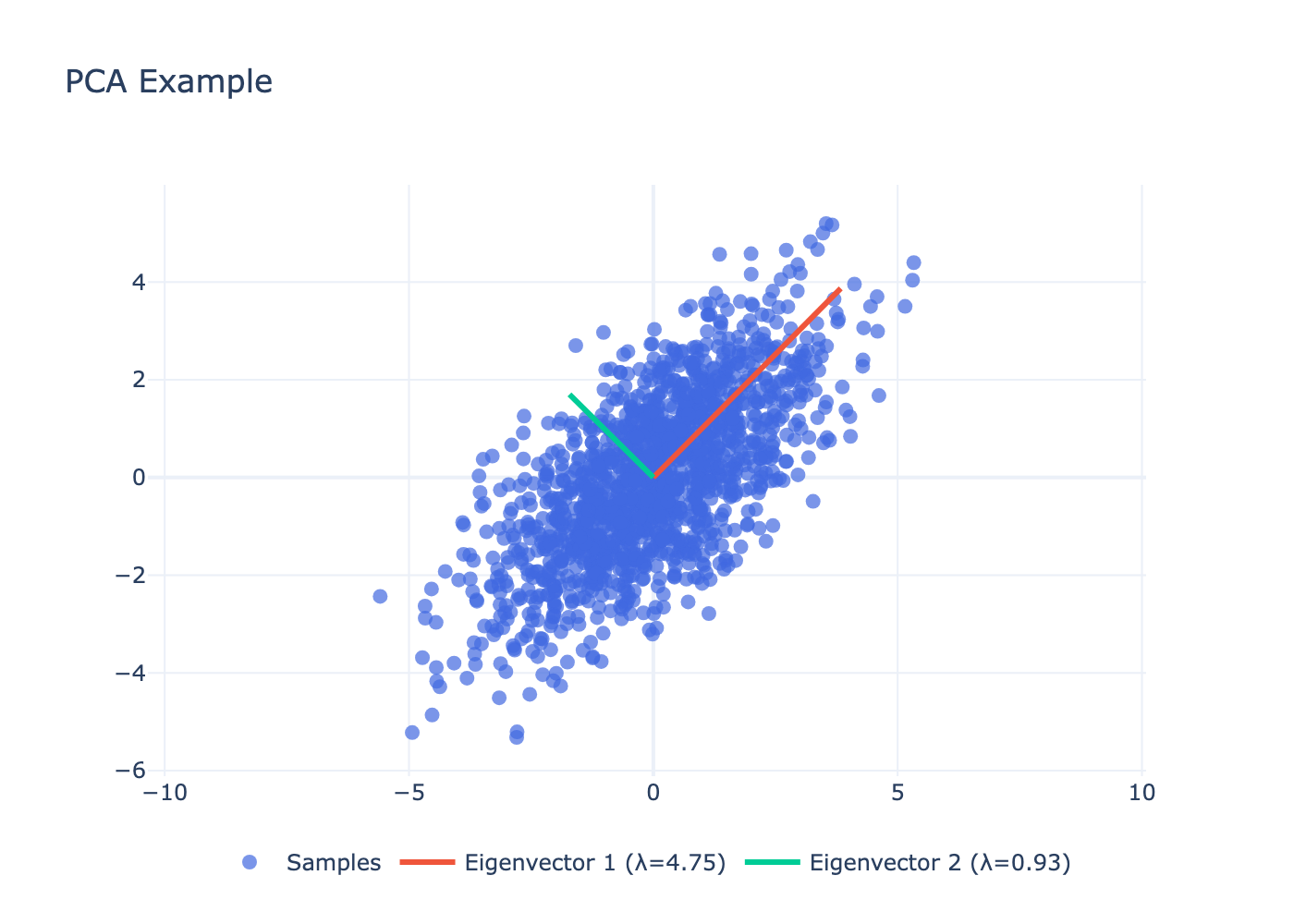
We generate a set of points with a specific correlation matrix. PCA has found the two main components that describe where the variance is. If you rotate by these vectors, you turn the samples into a cloud with unit noise. In this case, we have started with two dimensions and have two principal components, but it does not need to be one-to-one; you can have fewer principal components than dimensions.
In finance, this is a great technique because everything is so correlated. Assets are not moving completely independently; there are key factors. This is why PCA is the tool of choice. We are letting the data tell us the key elements rather than enforcing them ourselves.
PCA and FX
As always, Python, and specifically scikit-learn, has a simple method of calculating PCA on the data. For now, we are assuming five principal components. We have to drop the index and datetime columns so our data is just pure returns.
from sklearn.decomposition import PCA

r = returns.drop(["index", "datetime"])

pca = PCA(n_components=5)
pca.fit(r)

F = r @ pca.components_.T   # (T, K) — factor realisations
W = pca.components_
We are interested in how much variance each component explains.
pca.explained_variance_ratio_
array([0.42833194, 0.09363639, 0.04578692, 0.0385175 , 0.03270084])
This is a normalised measure of how much variation each component describes. So the first component explains 43%, the second factor 9%, and so on. It drops off quite significantly, so you can see why five components are enough for now, and more importantly, the first factor is such a large proportion.
To look at the weights, we can plot a heat map.
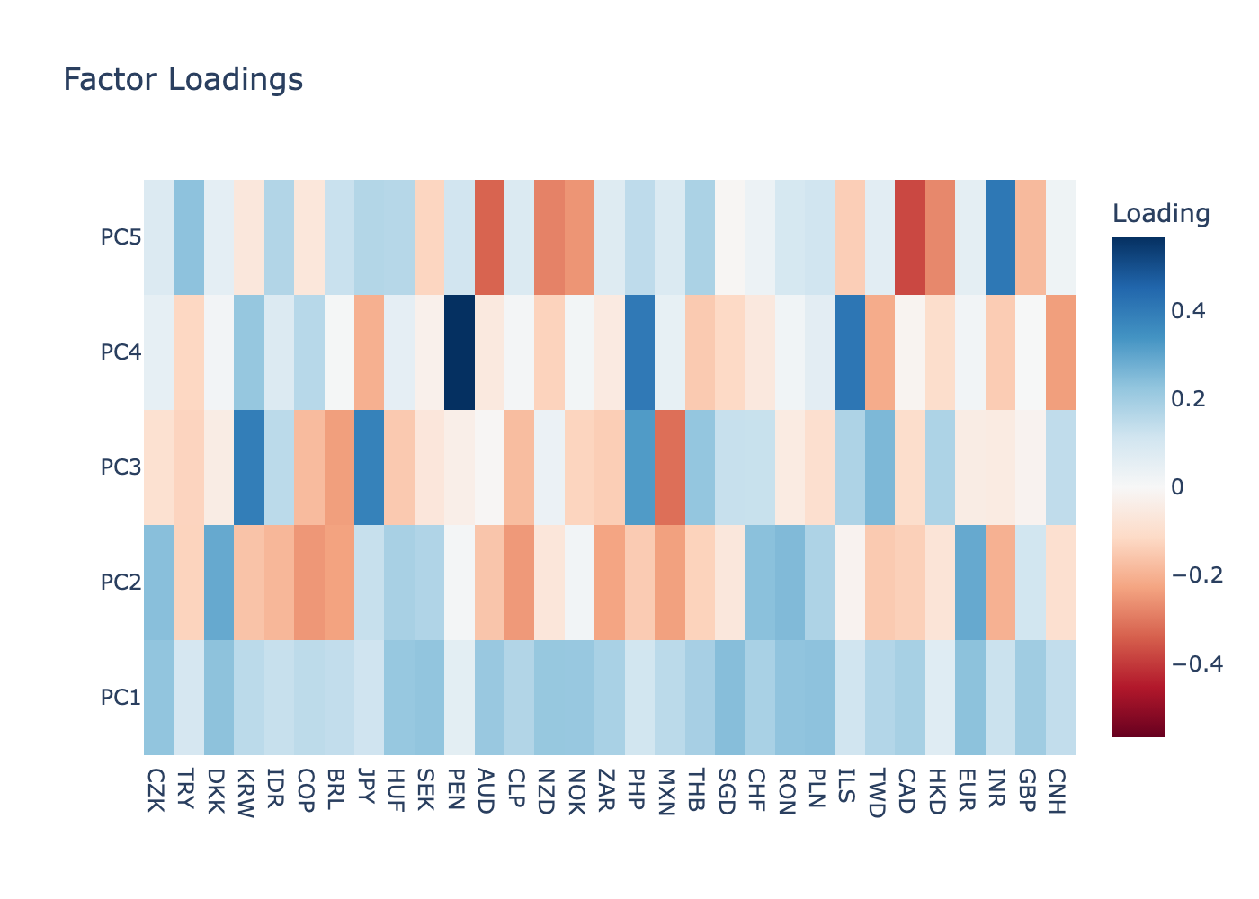
All the pairs in PC1 are positive. The first factor is the “market” factor, which in FX is most likely the dollar factor. This makes it the DXY equivalent. You could say it is better than the DXY because it contains more currencies and the weights are more reflective of the actual links between the currencies. The other factors are harder to interpret, but we will come back to this problem.
We can also look at the factor returns.
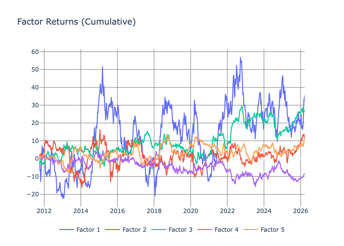
Factor 1 is very noisy but slowly drifting higher. Factor 3 has been positive since 2022, but all the others are oscillating around 0.
This is a good illustration of what PCA does on a dataset of returns, but it is completely useless for building a factor model. By using the entire dataset, we have committed the cardinal sin of back-testing and using information from the future. So, we need to adapt our PCA calculation to a rolling window. We did not have to worry about this in the fundamental model because StatsModels has the RollingOLS function.
Rolling PCA
We need to iterate through time and fit the PCA model using only data from the past to build up the weights correctly. It is simply a case of sliding a window along the data and fitting the PCA incrementally. There is some massaging of the PCA object to get the right data out, but overall it is fairly functional.
def rolling_pca(returns, window = 52, n_components = 4):

    assets = [c for c in returns.columns if c not in ("index", "datetime")]
    matrix = returns.select(assets).to_numpy()  # shape: (T, N)

    N = len(assets)
    T = matrix.shape[0]
    scores_out = np.full((T, n_components), np.nan)
    weights_out = np.full((T, n_components * N), np.nan)

    pca = PCA(n_components=n_components)

    for t in range(window - 1, T):
        window_matrix = matrix[t - window + 1 : t + 1]  # (window, N)

        if np.any(np.isnan(window_matrix)):
            continue

        scores = pca.fit_transform(window_matrix)  # (window, n_components)
        scores_out[t] = scores[-1]  # last row = current realisation, all components
        weights_out[t] = pca.components_.flatten()  # (n_components, N) -> (n_components * N,)

    score_cols = [pl.Series(f"factor_pc{i+1}", scores_out[:, i]) for i in range(n_components)]

    weight_cols = [
        pl.Series(f"weight_pc{i+1}_{asset}", weights_out[:, i * N + j])
        for i in range(n_components)
        for j, asset in enumerate(assets)
    ]
    return returns.select(["datetime"]).with_columns(score_cols + weight_cols)
Again, to keep it comparable to the fundamental model, we run it over a 52-week window but drop down to four components instead of the original five, given the explained variance plateau.
factor_df = rolling_pca(returns, window=52, n_components=4).drop_nans("factor_pc1")
This returns both the factors and the weights in a nice dataframe format with both the weights and the factors. Firstly, we look at the weights returned for the first component.
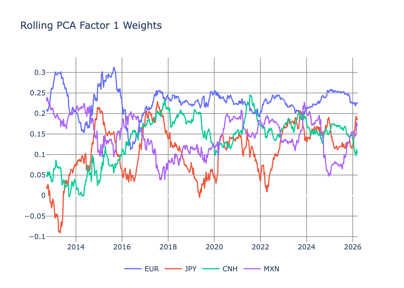
The key thing here is that the weights across the selected currency pairs are stable, and they are not changing from positive to negative frequently. This also lines up with our heatmap, which shows that all the weights in PC1 should be positive as the USD factor.
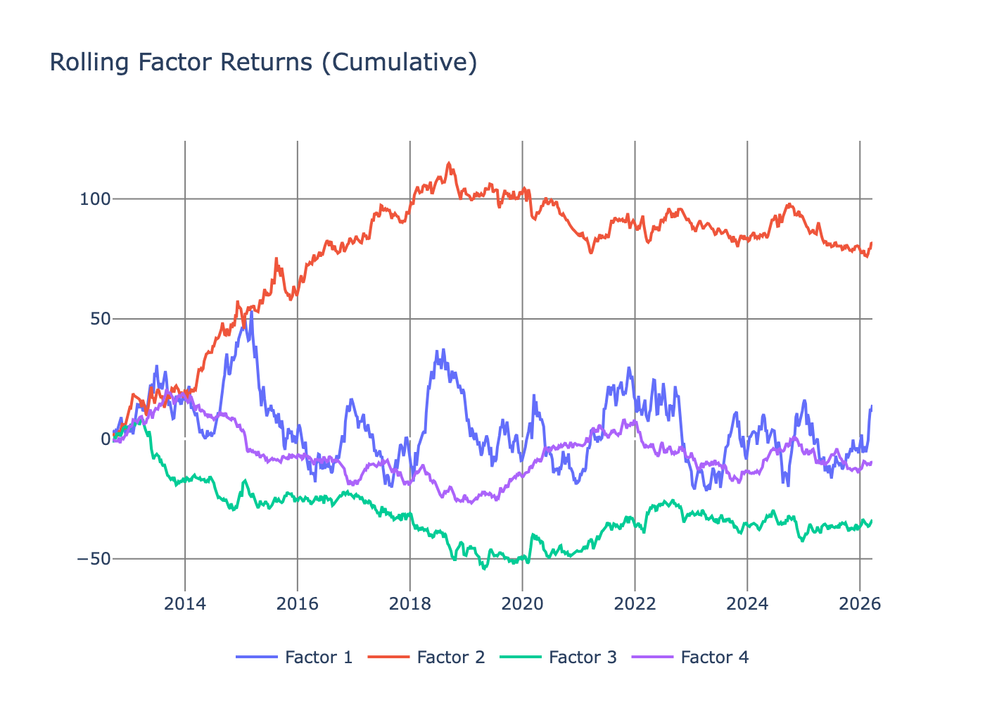
Looking at the returns across the four factors, we can see some differences. Firstly, factor 2 looks like a winner in the first four years, but has not done anything since 2018. All the others are fairly nondescript and oscillate around zero. Comparing it to the first PCA return plot, we can see how big a difference the data leakage made to the final results. So the rolling PCA is the right approach going forward.
This has given us the right format of factors to continue building out a factor model using the same steps as the fundamental model.
The \(\beta\) regression
Just like the fundamental factor model, we need to know how sensitive each currency’s individual return is to the different factors.
import statsmodels.formula.api as smf
from statsmodels.regression.rolling import RollingOLS

allParams = []

for ccy in ccys:
    subDF = df.filter(pl.col("ccy") == ccy).drop_nulls().sort("datetime")
    mod = RollingOLS.from_formula("log_return_scaled_clipped ~ factor_pc1 + factor_pc2 + factor_pc3 + factor_pc4",
                window = 52,
                data=subDF).fit()
    paramDF = pl.from_pandas(mod.params)
    paramDF = paramDF.with_columns(ccy=pl.lit(ccy),
                                   datetime = subDF["datetime"],
                                   log_return = subDF["log_return_scaled_clipped"],
                                   log_return_prev = subDF["log_return_scaled_clipped"].shift(1),
                                   r2 = mod.rsquared_adj.values,
                                   vol_52 = subDF["vol_52"])

    allParams.append(paramDF)

allParams = pl.concat(allParams).drop_nulls().sort("datetime")
Again, this is functionally the same model as the fundamental approach, just swapping out the ETF and momentum factors for these statistical factors. Looking at the average \(\beta\) values, we can see that the first factor is the only one with a real effect.
| variable | mean | std | min | max |
|---|---|---|---|---|
| factor_pc1 | 0.17 | 0.06 | -0.07 | 0.31 |
| factor_pc2 | 0.01 | 0.13 | -0.40 | 0.58 |
| Intercept | 0.01 | 0.09 | -0.41 | 0.38 |
| factor_pc3 | 0.01 | 0.12 | -0.40 | 0.59 |
| factor_pc4 | 0.01 | 0.13 | -0.42 | 0.57 |
The Factor Regression
Again, following the same process as the fundamental model, we now iterate through the dates and regress the returns across these \(\beta\) values. Scaling the \(\beta\) values across the currency pairs also helps normalise the regression results.
allParams2 = []

factor_cols = ["factor_pc1", "factor_pc2", "factor_pc3", "factor_pc4"]

for (i, dt) in enumerate(allParams["datetime"].unique()):
    subDF = allParams.filter(pl.col("datetime") == dt)

    subDF = subDF.with_columns([
    ((pl.col(c) - pl.col(c).mean().over("datetime")) /
      pl.col(c).std().over("datetime")).alias(f"{c}_scaled")
    for c in factor_cols
    ])

    csr = smf.wls("log_return_prev ~ factor_pc1_scaled + factor_pc2_scaled + factor_pc3_scaled + factor_pc4_scaled",
                  data=subDF, weights=1/(subDF["vol_52"]**2)).fit()

    paramsRes = pl.DataFrame(data = [[x] for x in csr.params.values],
             schema=list(csr.params.index.values))

    paramsRes = paramsRes.with_columns(datetime=pl.lit(dt))
    allParams2.append(paramsRes)

allParams2 = pl.concat(allParams2).drop_nulls().sort("datetime")
| variable | avg | std | N | std_error | t_stat |
|---|---|---|---|---|---|
| factor_pc4_scaled | 0.01 | 0.29 | 604 | 0.01 | 0.53 |
| Intercept | 0.01 | 0.61 | 604 | 0.02 | 0.50 |
| factor_pc3_scaled | 0.00 | 0.27 | 604 | 0.01 | 0.09 |
| factor_pc1_scaled | -0.00 | 0.31 | 604 | 0.01 | -0.20 |
| factor_pc2_scaled | -0.01 | 0.35 | 604 | 0.01 | -0.52 |
The key thing we are looking out for is any factor with a t-stat greater than 2. Unfortunately, none of the PCA factors have come out as significant. This means that none of the statistical factors can adequately explain the variation in returns across currencies. Again, this is a bit annoying but not surprising. So, given that these are the factors learned from the data, how are they correlated with the previous macro factors?
What Could the PCA Factors Be?
The factors that emerge from the PCA calculation are abstract. We need some way of judging what they could potentially represent. The easiest method is to bring back in the macro ETFs and the DXY to see how correlated they are with the new statistical factors.
This is all very simple, just left joins into the dataframe and use the inbuilt correlation calculation. We plot it as a heatmap to get a pretty visualisation.
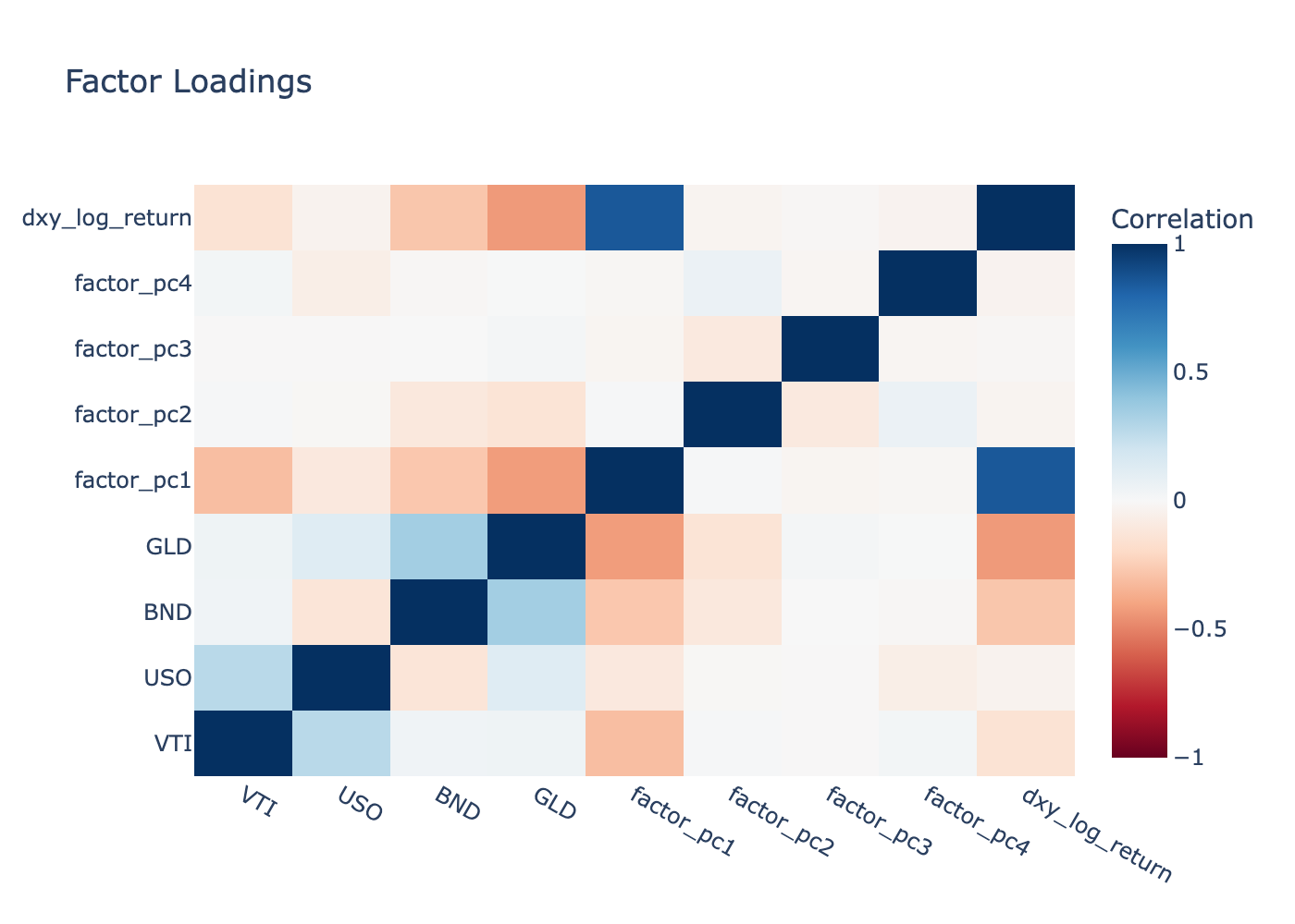
The only clear standout is PC1 with the DXY. This gives us some confidence in our work, as the first PCA component is always the market, and since I have spent two blog posts talking about the DXY as the market in FX, it is good to see that there is some statistical backing. Otherwise, the lack of correlation backs up the overall lacklustre results. There are no significant correlations between the rest of the factors and the macro ETFs.
Conclusion
If anything, this is less interesting than the fundamental model, as none of the statistical factors have come up significant. This comes down to the same caveats that I explained in that post: the small universe size, and FX just does not move as much as equities. Still, I hope you have learned an important lesson about data leakage and why you need to make sure you do not look backward. We have also shown that the first principal component and the DXY are very similar, so this could be a way to build a better DXY.
Overall, PCA is useful for discovering latent structure between the different currency pairs, but it hasn’t revealed any tradeable factors on its own.