Big Ticks and Small Ticks in Equity Microstructure
I bought Trades, Quotes and Prices a few years ago and it came with access to some free data to help you understand the concepts. That data was from LOBSTER and it has the limit order book (LOB) of five tech stocks for a single day in 2012. I did a quick top of book size calculation in Python and the liquidity profiles looked completely different. Intel and Microsoft had hundreds of thousands of dollars at the best prices, while Google and Amazon had only a fraction of that size. So my first thought was that the orderbook data needs some explaining and basic analysis before going into anything more complicated. In this post, we’ll cover how to load and parse LOBSTER data in Python, calculate core microstructure statistics, and explore how a stock’s tick size changes how it trades (big-tick vs. small-tick stocks).
Enjoy these types of posts? Then sign up for my newsletter.
You aren’t getting high-frequency market data for free. Exchanges sell this data and it must be worth something as people are willing to buy it. The big exchanges (NYSE, owned by ICE, and NASDAQ) make a significant amount of money selling their data and it is a revenue source that is continuing to grow. So what if you are a poor student who wants to play around with this data? Your options are limited, but you can either look at crypto (Using QuestDB to Build a Crypto Trade Database in Julia) or LOBSTER is kind enough to provide some sample data to get you on your way.
LOBSTER is an academic service that can provide full orderbook reconstruction from the raw NASDAQ market data. This creates a more familiar structure of both the orderbook snapshots at a given time and the messages from the exchange that have led to that orderbook. They have samples for GOOG, AMZN, MSFT, AAPL and INTC on one day. The files come as compressed CSVs, so no fancy or proprietary formats to worry about. This makes it all very easy to load into Python.
Parsing LOBSTER Order Book Data in Python
LOBSTER provides two file types: each individual message from the exchange and the subsequent order book that comes from the result of that message. You need both for the complete set of information, but that’s probably limited to joining across the timestamps.
We will be using Polars and so need the usual libraries.
import pathlib
import numpy as np
import polars as pl
import polars.selectors as cs
The LOBSTER Message File
This is a simple CSV with six columns, with one file per ticker.
def load_message(ticker):
    colnames = ["time", "event_type", "order_id", "size", "price", "direction"]

    messageFile = sorted(pathlib.Path('LOBSTER/').glob(f'**/{ticker}_*message_10*.csv'))

    message = pl.read_csv(messageFile[0],
                       has_header=False)
    message = message.rename(dict(zip(message.columns, colnames)))
    return message
The LOBSTER Orderbook File
This is a wider file with four columns for each level, detailing the bid/offer price and size.
def load_orderbook(ticker):

    colnames = [[f"ask_price_{i}", f"ask_size_{i}", f"bid_price_{i}", f"bid_size_{i}"] for i in range(1, 11)]
    colnames = np.array(colnames).flatten().tolist()

    orderbookFile = sorted(pathlib.Path('LOBSTER/').glob(f'**/{ticker}_*orderbook_10*.csv'))

    orderbook = pl.read_csv(orderbookFile[0],
                       has_header=False)
    orderbook = orderbook.rename(dict(zip(orderbook.columns, colnames)))
    return orderbook
Bringing It All Together
def load_ticker(ticker):

    orderbook = load_orderbook(ticker)
    message = load_message(ticker)
    orderbook = orderbook.with_row_index().join(message.with_row_index(), on="index", how="left")

    price_cols = orderbook.select(cs.contains("price")).columns

    orderbook = orderbook.with_columns(
        [pl.col(c) * 1e-4 for c in price_cols]
    )

    orderbook = orderbook.with_columns(
        ticker=pl.lit(ticker),
        date=pl.lit("2012-06-21")
    )
    return orderbook
Prices are multiplied by 10,000, so we need to undo that to get the correct prices. The sample date they provide is 21 June 2012, so it’s useful to add that in too.
So, what we end up doing is loading the full order book for each ticker and bringing it all together into one big data frame.
orderbook = pl.concat([load_ticker(ticker) for ticker in ["AAPL", "MSFT", "GOOG", "AMZN", "INTC"]])
Then, to add in the timestamp of each event, we parse the date and time column.
orderbook = orderbook.with_columns(
    timestamp =(pl.col("date").str.to_datetime("%Y-%m-%d").dt.replace_time_zone(None) +
     pl.duration(nanoseconds=(pl.col("time") * 1e9).cast(pl.Int64)))
)
We are now ready to go and can calculate some microstructure statistics.
Calculating Core Market Microstructure Metrics
From the order-book data, we can now calculate some basic statistics for the different stocks. I’ve previously looked at microstructure noise with Hawkes processes and order flow imbalance, here we are focusing on static order book snapshots. We want to understand how the order books differ across stocks and what consequences that has for how cheap or expensive it is to trade them.
We need to first calculate the spread, which is the difference between the best prices you can buy and sell at, and also the top-of-book size (tob_size), which is the average amount you can trade at the best prices. We also add in the mid-price and how long the quote was alive for. Using the mid-price, we can convert the spread into percentage points (or basis points, bps).
orderbook = orderbook.with_columns(
    spread = pl.col("ask_price_1") - pl.col("bid_price_1"),
    tob_size = 0.5*(pl.col("ask_size_1") + pl.col("bid_size_1")),
    mid_price = 0.5*(pl.col("ask_price_1") + pl.col("bid_price_1")),
    quote_duration = (pl.col("time").shift(-1) - pl.col("time")).fill_null(0).over("ticker")
    )

orderbook = orderbook.with_columns(
    spread_bps = 10000*pl.col("spread")/pl.col("mid_price")
    )
With all these variables calculated, we can start calculating some averages.
Top of Book Size
This is the number of shares that you can trade at the best price (to buy or sell). It should be clear that the larger this is, the cheaper it is to trade, because you can get more done at the best price available. We are taking a duration-weighted average and also multiplying it by the mid-price to calculate the notional amount.
res = orderbook.group_by("ticker").agg(
    mid = pl.col("mid_price").mean(),
    wavg_tob_size = (pl.col("quote_duration").dot(pl.col("tob_size")))/pl.col("quote_duration").sum()
    )

res = res.with_columns(
    dollars_tob = pl.col("wavg_tob_size")*pl.col("mid")
    )
| ticker | wavg_tob_size | dollars_tob |
|---|---|---|
| AAPL | 153.75 | $89,660.17 |
| INTC | 14018.53 | $379,245.55 |
| MSFT | 11557.95 | $353,083.24 |
| GOOG | 156.68 | $89,429.38 |
| AMZN | 178.60 | $39,777.11 |
When we measure it just by the number of shares, we can see a stark difference between MSFT and INTC versus the others, as there is an order-of-magnitude difference in the number of shares available. If we multiply the number of shares by the average mid-price, we can measure the dollar amount of shares available to execute at the best price. There is still a large difference, but it is closer in order of magnitude (hundreds of thousands of dollars).
Top of Book Spread
This is the distance between the two top-of-book prices. We measure it in basis points (bps). There is a bit more nuance in what this means for trading costs, but there are different ways to think about it. First, it is simply the difference between what you can buy and what you can sell. This can quantify the overall round-trip cost if you bought some stock and then sold it later, i.e. how much money you would lose.
From our data across the stocks, we take the time-weighted average of the spread. You can measure it with different units.
- Raw price increments, \(\text{ask} - \text{bid}\),
wavg_spread. - In basis points, \(1e4 \cdot \frac{\text{ask} - \text{bid}}{\text{mid}}\),
wavg_spread_bps. This is a percentage measure where 1 bp = 0.01%. - In ticks, \(\frac{\text{ask} - \text{bid}}{\text{tick size}}\),
spread_ticks.
res = orderbook.group_by("ticker").agg(
    min_spread = pl.col("spread").min(),
    wavg_spread = (pl.col("quote_duration").dot(pl.col("spread")))/pl.col("quote_duration").sum(),
    wavg_spread_bps = (pl.col("quote_duration").dot(pl.col("spread_bps")))/pl.col("quote_duration").sum()
    )

res = res.with_columns(
    spread_ticks = pl.col("wavg_spread")/pl.col("min_spread")
)
| ticker | min_spread | wavg_spread | wavg_spread_bps | spread_ticks |
|---|---|---|---|---|
| AAPL | 0.01 | 0.15 | 2.59 | 15.13 |
| INTC | 0.01 | 0.01 | 3.75 | 1.01 |
| MSFT | 0.01 | 0.01 | 3.31 | 1.01 |
| GOOG | 0.01 | 0.27 | 4.78 | 27.33 |
| AMZN | 0.01 | 0.13 | 5.76 | 12.85 |
There is not quite as much of a difference between the stocks here; the basis-point measure is between 2 and 6. There is a structural difference when measuring the spread in ticks: MSFT and INTC are as tight as they can possibly be, whereas the others have some room to improve on average.
Depth of Book Size
Now we are looking beyond the first level. This is the total size across the 10 levels we have access to. The logic here is that more size on the order book overall means you can actually get more done overall without having to wait for liquidity providers to replenish the order book after the initial liquidity has been removed. So we take the average size at each of the 10 levels, normalise by the TOB size, and plot the overall shape.
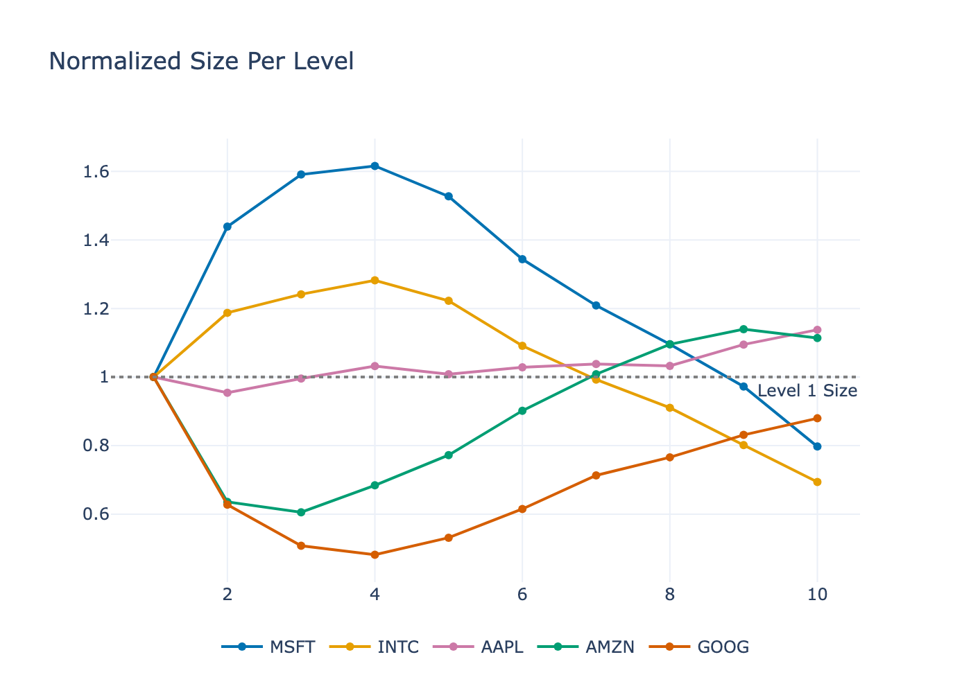
We end up with two different shapes. AMZN and GOOG have less liquidity than the top of book at intermediate levels, whereas MSFT and INTC see more size at the intermediate levels. AAPL is pretty constant through the 10 levels.
Depth of Book Cost
The depth of book cost adds another dimension to the depth of book size. This is no longer a single number but a curve that shows how much it would cost to trade a specific amount while also giving some sense of interpolation between sizes. I have done a similar calculation for cryptocurrencies with my pre-trade tool - cryptoliquiditymetrics. As the sizes are so different across the stocks, I had to group by the deciles when calculating the costs.
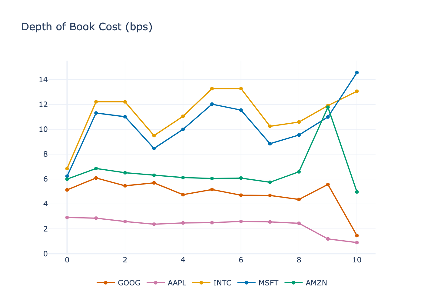
This graph shows how much in basis points it will cost you to trade through the book. INTC and MSFT see the expected growth in cost as size increases; all the others are pretty flat which is a bit surprising. But that brings me onto the next topic. There have now been multiple microstructure statistics where MSFT and INTC are different to the other three and this is how the exchange has set them up to trade.
Big Tick vs Small Tick
If we look again at the average spread table, but focus just on the ticks column:
| ticker | min_spread | spread_ticks |
|---|---|---|
| AAPL | 0.01 | 15.13 |
| INTC | 0.01 | 1.01 |
| MSFT | 0.01 | 1.01 |
| GOOG | 0.01 | 27.33 |
| AMZN | 0.01 | 12.85 |
MSFT and INTC are on average a single tick wide. This means that anyone submitting an order can never improve on either the bid or ask, because there is no space in between the best bid or offer—it is tick-constrained. For the other three stocks, the spread is at least 10x the minimum tick size, so there is always space to submit a better price than the one currently displayed.
- MSFT and INTC are big-tick stocks; their tick size is large compared to the bid/offer spread.
- GOOG, AMZN, and AAPL are small-tick stocks; their tick size is small relative to the average spread.
This simple difference explains most of the above microstructure differences. Big-tick stocks have a heavy top-of-book size and tighter spreads (in bps terms), which is true for MSFT and INTC relative to GOOG and AMZN. AAPL is an exception here: its high nominal share price (~$580) means its spread in basis points is very small (2.59 bps) despite spanning roughly 15 ticks. Technically, the real spread for MSFT and INTC should be tighter; the tick size is getting in the way of people displaying their true interest. Instead, it is a game around queue priority: for big ticks, if the price changes you want to be first in the queue at the new price; for small ticks, you can just jump the queue by posting inside the spread.
For the depth of book size, we saw a large difference between AMZN/GOOG and MSFT/INTC. Again, this is due to the tick size. Big ticks show lots of size at multiple levels, whereas small ticks are thinner at each level.
This all comes down to specific US rules (Reg NMS Rule 612 — the Sub-Penny Rule), which dictates that any stock with a price greater than a dollar must have 1 cent as its minimum tick size. This dataset was from 2012, when MSFT and INTC traded at $30 and $27, respectively, while GOOG and AAPL traded at $570 and $583. That is an order-of-magnitude difference in price, but the exact same tick size. One cent is a rounding error for GOOG and AAPL but much more significant for MSFT and INTC.
The SEC addressed this tick-constrained problem by adopting amendments to Regulation NMS to establish a smaller, half-cent ($0.005) tick size for tick-constrained stocks with tight spreads. Under the rule, if a stock’s time-weighted average quoted spread is $0.015 or less over a 3-month evaluation period, it can move to a half-penny minimum quoting increment. The market is showing that it wants to quote tighter and this new rule lets it happen.
It gets even more interesting because this ruling applies to public exchanges (like NASDAQ and the NYSE). Dark pools and wholesalers—i.e., the payment for order flow (PFOF) players—have already been able to quote and fill at sub-penny prices off-exchange. Equity microstructure, an entirely different beast compared to my usual currency stuff!
Conclusion
This has been a whistle-stop tour of some basic equity microstructure, but mainly shows how the tick size can have a large effect on the actual economics of trading. Not all stocks trade in the same way, even when they are fundamentally similar and on the surface you wouldn’t expect such a difference in behaviour. These mechanics are essential to any type of trading strategy, from an execution algorithm to a price impact model. It all basically comes down to whether you are competing by price (small tick) or competing by queueing (big tick).
Finally, I managed to write all that without a single big tick energy joke.